Evaluation of Methods for Detecting and Locating Faults in HVDC Grids

(1)

Evaluation of Methods for Detecting and

Locating Faults in HVDC Grids

Erik Martinsen

Master of Energy and Environmental Engineering Supervisor: Hans Kristian Høidalen, ELKRAFT Co-supervisor: Salvatore D'Arco, SINTEF

Department of Electric Power Engineering Submission date: June 2014

(2)

(3)

Problem description

Protection in HVDC networks is more difficult than in AC networks, both due to the low impedance and lack of changes in current polarity. Very fast tripping of DC interruption devices is required in order to avoid harmful stress to the converters. A project at SINTEF energy Research addresses protection and fault handling in offshore DC grids, but with main focus on power converter performance.

In order to investigate different protection principles, a simple Multi Terminal High Voltage Direct Current (MTDC), radial cable based system is to be modeled in PSCAD. Simulation models are obtainable from SINTEF, but this should be tested and extended. The model should incorporate full switching, two level voltage source converters and a cable model suiatble for simulations of direct current. The finished model is to be used for investigating fault currents and voltages in the MTDC system.

Once fault characteristics have been established, different fault localisation prin-ciples shall be implemented in the MTDC system model. Traditional methods which should be considered for implementation include:

• Overcurrent and undervoltage protection • Differential protection

• Voltage derivative protection

In addition, newer localisation methods based on signal processing should also be investigated, especially the following two methods:

• Travelling wave protection

• Fault location algorithms, for instance Wavelet transforms

Goal of the project is to implement these methods in the PSCAD model and evaluate them under different fault conditions. Following this evaluation, a pro-tection scheme which will meet requirements for fast and precise fault depro-tection and localisation for all faults should be implemented if possible.

(4)

(5)

Abstract

In this thesis work, different proposed methods for detecting and locating short circuit faults in Multi Terminal HVDC grids have been evaluated by implemena-tion and transient simulaimplemena-tions in PSCAD. The research has been limited to cable based systems.

HVDC grids have seen increasing interest in recent years, but have yet to be fully realised. Suitable converter technology was introduced in 1997 and has been further developed since, while switches able to interrupt large DC currents were introduced in June 2013. One of the major issues left is fault localisation. Due to the low impedance in HVDC cable systems, fault currents rise to severe magnitudes system wide in a matter of a few milliseconds. This may cause damage to the converter diodes if not dealt with quickly.

In order to obtain a better understanding of the fault propagation, research into the subject is presented. It is found that the capacitors in the converters is a main source of large fault currents, and fast fault detection is essential for protec-tion of converter components. Time between first detecprotec-tion of fault until current interruption should be within a few milliseconds.

Different methods have been proposed for localisation of faults in recent years. These are presented together with traditional fault localisation methods, and briefly discussed with the intent of deciding which to implement and evaluate in PSCAD.

Protection based on current derivative and wavelet transformation, as well as travelling wave protection is chosen and implemented in a three converter VSC system. Different fault types are applied at various locations with varying system capacitance and up to 16 fault impedance. The results indicate that none of the three methods are able to detect and locate all impedance faults on their own. The travelling wave protection is suitable for short lines, but fails when exposed to high fault impedances and distances.

By using derivative polarity to determine direction of fault and wavelet magnitude to determine distance, faults are successfully located in a high capacitance system within a respectable time. It is concluded that all the three tested methods should be considered for implementation when designing a future HVDC protection sys-tem.

(6)

Sammendrag

I denne avhandlingen er forskjellige foresl˚atte metoder for ˚a bestemme feillokasjon i flerterminals HVDC systemer presentert og undersøkt ved hjelp av simuleringer i PSCAD. Simuleringene har tatt for seg et radielt kabelsystem med tre VSC omformere.

Interessen for flerterminals HVDC systemer har økt de siste ˚arene, men et større system har enda ikke blitt realisert. Passende omformerteknologi ble innført i 1997 og har blitt utviklet videre i senere tid. Brytning av store likestrømmer har lenge vært umulig, men ny bryterteknologi med dette form˚alet ble introdusert i juni 2013. En av de største gjenværende utfordringene er feillokalisering. P˚a grunn av lav impedans i kabelbaserte HVDC systemer stiger feilstrømmer raskt til niv˚aer som kan for˚arsake skade p˚a komponenter i systemet.

For ˚a oppn˚a en bedre forst˚aelse av hvordan feil sprer seg i nettet blir nyere forskn-ing p˚a feltet presentert. Det konkluderes med at filterkapasitansen i de nye om-formerne er en hoved˚arsak til store feilstrømmer, og rask feillokalisering er essen-sielt for ˚a unng˚a skade p˚a komponenter i omformerne. For ˚a unng˚a dette bør feilen klareres innen f˚a millisekunder.

Forskjellige metoder for ˚a gjennomføre feillokalisering i HVDC nett p˚a en rask og sikker m˚ate har blitt foresl˚att i nyere tid. Noen av disse er presentert sammen med tradisjonelle metoder for feillokalisering med det form˚al ˚a bestemme hvilke som skal implementeres i PSCAD.

Lokaliseringsmetoder basert p˚a derivering av strøm, wavelet transformasjon og vandrebølger blir implementert i et radielt HVDC system med tre VSC omformere. Forskjellige feiltyper blir lagt inn ved forskjellige lokasjoner i nettet, med vari-erende kapasitans ved omformerne og opptil 16 feilimpedans. Resultatene in-dikerer at ingen av de tre systemene kan lokalisere feilen p˚a egenh˚and, uavhengig av feilimpedans og avstand til feil. Vandrebølgemetoden er egnet for linjer med begrenset lengde, men klarer ikke ˚a oppdage feil over lengre distanse med høy impedans.

Ved ˚a benytte polariteten til den deriverte av strømmen for ˚a bestemme feilretning og wavelet koeffisienten til ˚a bestemme avstand lykkes det ˚a detektere feil raskt og sikkert i et system med høy kapasitans for alle feildistanser og –impedanser. Alle de tre systemene anses som egnet til ˚a være del av en endelig lokaliseringsløsning for HVDC nett.

(7)

Acknowledgements

There are many who deserve thanks for helping me through the last five years of studying, and especially with the last semester of writing this thesis.

First of all I must thank my two supervisors, professor Hans Kristian Høidalen at NTNU and Salvatore D’Arco at SINTEF Energy, for this interesting and chal-lenging work. You have laid the foundation and supported me in uncertain times, and been there for me when I had questions.

A big thank you also goes to other employees at SINTEF energy, namely John Are Suul and Andrzej Holdyk who have provided me with the necessary simulation models and always been available for explanations of difficult questions.

I must also thank my fellow students at NTNU and the city of Trondheim for good times and many wonderful memories. Especially those I have been spending most time with. Ole, Marielle, Truls, Richard and Hanne, it would have been awfully boring without you.

Lastly, I thank my father and brother who always believe in me, even when I do not.

Trondheim June 2014 Erik Martinsen

(8)

(9)

List of Figures

2.1 The Quebec-New England MTDC transmission line. . . 6

2.2 Proposed topology for MTDC system in the North Sea. . . 7

2.3 Different grid topologies . . . 8

2.4 Asymmetric monopoles with three converters . . . 10

2.5 Symmetrical monopole with grounded midpoint and earth return . 11 2.6 Bipolar system with grounded midpole and metallic return . . . 11

2.7 Asymmetric monopole connected to a two converter bipolar system 13 2.8 6-pulse Current Source Converter - Arrangement of thyristors . . . 14

2.9 6-pulse Voltage Source Converter - Arrangement of transistors . . . 15

2.10 The full bridge VSC for connection to a single phase. . . 16

2.11 Five-level VSC phase leg . . . 17

2.12 The modular multilevel converter, placement of submodules (SM) . 18 2.13 Design of half bridge MMC sub module . . . 18

2.14 The full bridge sub module as proposed in . . . 19

2.15 The clamped double sub module as proposed in . . . 19

2.16 Cable cross section. . . 20

2.17 The DC circuit breaker designed by ABB. . . 21

2.18 The concept of a tuned LC circuit . . . 23

2.19 PTC during normal operation and at fault . . . 23

3.1 A simple resistive system with fault . . . 26

3.2 A capacitive system with fault . . . 26

3.3 Discharge voltage and current of RC circuit with varying resistance 27 3.4 A pi-equivalent . . . 29

3.5 A series RLC circuit . . . 29

3.6 Natural response of an RLC circuit . . . 31

3.7 Wave initialized at ground fault . . . 32

3.8 Wave reflected at converter . . . 32

3.9 Lattice diagram showing how waves are reflected between two con-verters and fault point . . . 33

3.10 Wave approaching a VSC station with neighbouring line connected 34 3.11 Build up of current at converter shown together with the Lattice diagram over arriving waves . . . 35

3.12 Fault current development in MTDC grid for different system topolo-gies . . . 36

3.13 The three stages of fault development . . . 37 ix

(14)

3.14 Two converter system with fault between the converters . . . 37

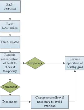
3.15 The process from detecting fault to normal operation is resumed . . 40

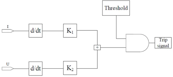
4.1 Operational process of voltage derivative protection . . . 44

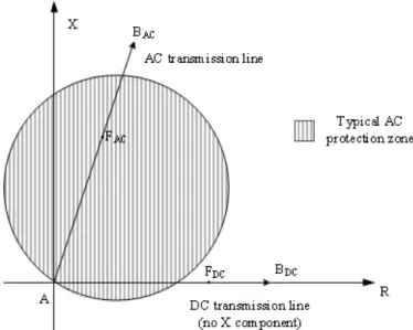
4.2 Typical R-X characteristic of a transmission line . . . 46

4.3 Haar and Daubechies mother wavelets . . . 50

4.4 Forward Feeding Artificial Neural Network structure . . . 52

5.1 The MTDC system implemented in PSCAD with all measurement and fault points indicated . . . 55

6.1 Layout of the implemented MTDC system . . . 64

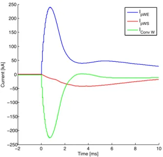
6.2 Voltage and current recordings during fault at pos WE1 . . . 65

6.3 Current in breakers pWE and pWS, with current from converter W 66 6.4 Currents in healthy lines during nearby faults . . . 67

6.5 Frequency analysis of current on the positive pole WE line during fault at pos WE1 . . . 67

6.6 Frequency analysis of current in breakers pWS and pSW during fault at pos WE1 . . . 68

6.7 Influence of filter capacitance on the fault currents and voltages. Fault location pos WE1 . . . 69

6.8 Frequency content of current IpW S for fault at pos WS1 . . . 70

6.9 Voltage and current recordings from converter W during positive pole fault at location WE1 under varying fault impedance . . . 70

6.10 Frequency analysis for different fault impedances . . . 71

6.11 Diode currents with a converter capacitance of 631.36 µF . . . 72

6.14 Wavelets recorded during fault at pos WE1 . . . 73

6.15 Wavelet analysis of fault currents following a fault at pos WE1. Recorded in pWE with varying filter capacitance . . . 75

6.16 Wavelet analysis of fault currents following a fault at pos WE1. Recorded at converter W with varying filter capacitance . . . 76

6.17 Recorded derivatives during a positive pole fault at WE1 . . . 77

6.18 Negative derivative value just prior to arrival of transient wave at converter . . . 78

6.19 Derivatives recorded after fault 40 km from converter S . . . 79

6.20 Fault derivatives with varying filter capacitance. Fault pos WE1 . . 79

6.21 Derivatives at converter W, fault pos WE1, varying fault impedance 80 6.22 Detailed current development in the positive pole of line WE . . . . 81

6.23 Currents with fault impedance of 16 ohm and high fault distances . 82 6.24 Voltage and current recordings after tripping converter W . . . 83

6.25 Derivatives and wavelets recorded after tripping converter W . . . . 84

6.26 Voltages and currents following change in voltage reference at con-verter W . . . 84

(15)

List of Figures

6.27 Voltages and currents recorded after a change in power reference at converter S . . . 85 7.1 Decision algorithm for fault detection based on wavelet and

deriva-tive measurements . . . 93

(16)

(17)

List of Tables

2.1 Advantages and disadvantages with different grid topologies . . . . 8

3.1 Criteria for damping of RLC circuit . . . 30

5.1 AC system parameters . . . 56

5.2 Cable materials . . . 57

5.3 Cable dimensions . . . 57

5.4 Cable resistance, capacitance, inductance and wave impedance . . . 57

5.5 Variation of parameters in different simulation cases . . . 60

5.6 Distance, resistance, total line inductance and capacitance between each converter and fault points . . . 61

5.7 Values for damping ratio at different fault impedances . . . 61

6.1 Wavelet peaks compared to filter capacitance . . . 75

7.1 Maximum values detected for faults within protection zone with large fault path impedance . . . 92

7.2 Maximum wavelet and derivative values detected for faults outside protection zone . . . 94

7.3 Derivative and wavelet thresholds for each of the breakers . . . 94

(18)

(19)

Abbreviations

HVDC High Voltage Direct Current HVAC High Voltage Alternating Current

MTDC Multi Terminal High Voltage Direct Current MMC Modular Multilevel Converter

HBSM Half Bridge SubModule FBSM Full Bridge SubModule

C-DSM Clamped-Ddouble Sub Module VSC VoltageSource Converter CSC Current Source Converter ANN ArtificialNeural Networks OCT OpticalCurrent Transducer

(20)

(21)

Chapter 1

Introduction

1.1 Background and motivation

With the ever increasing demand for electrical power and construction of renew-able energy, there is a need for increased power transmission capacity over long distances. Implementing the increased power generation into an existing power system, such as in Europe or North America, represents a challenge for the ma-ture HVAC network [1]. To overcome this challenge, increased interconnection of load centers with the use of HVDC has been proposed as an efficient and eco-nomical solution. Classic HVDC systems are point-to-point systems, but great advantages could be obtained by the implementation of an interconnected HVDC grid [2].

For the implementation of a full HVDC grid, voltage Source Converters (VSCs) are favored over traditional Current Source Converters (CSCs) [1]. This is pri-marily due to the VSCs capability of changing power flow by reverting current direction, as opposed to the CSC which changes voltage polarity. However, there are several challenges related to the development of a multi-converter, complex HVDC grid based on VSCs. Amongst the most serious of these is fault handling [2]. The low impedance in HVDC grids coupled with the lack of changing current polarity makes both locating and interrupting a fault more difficult than in HVAC networks. Compared to a CSC, the VSC has a very low inductance, making it more susceptible to damage during DC faults.

(22)

For the last decade, several methods for locating DC short circuit faults have been proposed. While there are some very promising solutions, very few have been tested for various fault locations and fault types. When implementing a fault detection system, it is important to know that the system will be able to detect all faults regardless of fault location and impedance. It is also of interest to determine what system parameters limits the implementation of the different systems.

1.2 Scope and limitations

For this thesis, different proposed fault localisation methods will be presented. Some of the presented methods are implemented in a computer model of a power system in PSCAD. Faults will be applied at various locations and with varying fault impedance. In addition, parameters of the grid which may affect the results are varied.

There are multiple goals with the simulations. First, the simulated fault currents and voltages will be compared to results obtained in previous literature to confirm the behaviour of the model. Second, the results will determine how the different methods perform under different conditions. It is especially interesting to deter-mine weaknesses and limits of each method. Lastly, the results will be used to propose a detection system using one or more of the implemented methods. The simulations and investigations are limited to detecting and locating the fault. Current interruption and isolation of fault will not be simulated, merely discussed. The implemented model does not contain any overhead HVDC lines, only cables. Overhead lines have different characteristics than cables, including higher induc-tance and lower capaciinduc-tance, which will influence fault behaviour.

Faults are only applied in DC cables and the converters. It will not be tested whether the different methods are able to differentiate between AC and DC faults, nor are the effects of DC faults on the AC system investigated.

(23)

1.3. Thesis structure 3

1.3 Thesis structure

The thesis is structured in 8 chapters and five appendices, following this introduc-tion which is the first chapter.

The second chapter describes how the HVDC grid can be built, with an emphasis on the components and different construction schemes. This is based on literature regarding classic HVDC systems as well as various studies into the feasibility of HVDC grids.

In the third chapter, theory regarding fault currents is introduced. Results from several papers which have investigated faults in HVDC grids are also presented. Emphasis is on determining how fast a protection system must act to avoid system damage, and also what parameters influences the fault currents.

In the fourth chapter, different methods for fault detection are presented, and evaluated for use in HVDC systems. Both traditional and newly proposed fault location methods are examined, and some of these are later picked for implemen-tation in PSCAD.

The fifth chapter describes the implemented PSCAD model and detection methods together with the planned simulations and expectations of results.

The sixth chapter contain results from the simulations, and also explanations to some of the observations, as well as a discussion of the different detection methods. Based on the results in chapter six, the possibility of a detection system based around those methods is discussed in chapter seven.

Conclusions and proposal for further work are then presented in chapters eight and nine.

1.4 Procedure for writing the thesis

The basis of this thesis will be the results obtained from simulations of faults in PSCAD. PSCAD is a very advanced and widely used power transient simulation software, containing one of the worlds most accurate cable models for simulating power transients. The implemented VSC model is provided by SINTEF energy

(24)

research, including the control system. SINTEF has also provided parameters for the cable model.

In order to plot the results in a presentable manner, MATLAB is used to process the results from PSCAD. MATLAB is also used for other forms of post-processing, which will be detailed in chapter five.

A literature study into the construction of HVDC grids, fault propagation, and fault detection in HVDC grids was undertaken prior to writing this thesis. This work forms the main body of chapters two through four.

(25)

Chapter 2

The Multi terminal HVDC

system

2.1 History of HVDC and the road to an HVDC

grid

HVDC systems have a long history in electrical engineering. In the early age of electricity, all distribution systems were DC. However, as the electrical grid grew there was an increasing demand for higher voltage and power levels, making HVAC systems the norm [1]. In more recent years however, HVDC systems have seen an increase in popularity, and is a popular choice for several applications. These are mainly bulk power transmission across long distances, and the interconnection of HVAC systems operating at different frequencies from one another, known as asynchronous networks [1]. HVDC is also often preferred over HVAC for use in cables, as this drastically decreases voltage loss.

So far all HVDC systems, with a few exceptions, are point to point systems, mean-ing the power transfer is merely between two converter stations, either connected with cable or overhead line. With recent increase in power demand and produc-tion, and especially the increasing renewable share, serious effort has been devoted to examine the feasibility of more complex HVDC systems with several converters interconnected. Such a system is known as a Multi Terminal HVDC (MTDC) system. There are a few in current operation, with the three converter Canadian

(26)

Figure 2.1: The Quebec-New England MTDC transmission line. Taken from [3]

Quebec-New England connection being amongst the first. This is illustrated in figure 2.1, albeit two of the converters shown are no longer in operation [1]. The future HVDC grid is envisioned to fulfil a larger amount of different tasks than the traditional HVDC connections. Some of these are presented in [1]:

• Supply power to urban load centres

• Interconnection of offshore installations, especially wind farms and oil/gas

platforms

• Bulk power transfer between countries and continents

An HVDC grid can be imagined both as an independent grid, or as an overlay grid alleviating the strain on existing HVAC grids which are close to their maximum operating point [1]. There are several advantages for choosing HVDC over HVAC for the future expansion of the high voltage power transmission [1]:

• Lower number of cables and reduced visual impact • Enables power exchange between asynchronous networks • Lower losses over long distances

(27)

2.1. History of HVDC and the road to an HVDC grid 7

Figure 2.2: Proposed topology for MTDC system in the North Sea. Dotted lines are existing HVDC interconnections. Taken from [2]

However, there are technical challenges which must be overcome before the real-isation of MTDC systems is feasible. Important steps have been made in recent decades, especially with the introduction of new converter technology in 1997 by ABB [4], known as Voltage Source Converter (VSC). Among the remaining chal-lenges, fault handling is considered one of the major ones [2, p. 83] [1, 5].

The possibility of a European HVDC supergrid has been investigated in [2], where different design possibilities are discussed. Different system topologies for an MTDC system in the North Sea are proposed, one of which is illustrated in figure 2.2. Varying power and voltage ratings are also proposed. Due to constraints in development of converter technology, it is assumed that power rating in a VSC based network will be limited to 1.2 GW until year 2020, and increase to 2 GW in the year 2030. Voltage rating for the 1.2 GW system is proposed to ±320 kV,

and increased to ±500 kV for a 2 GW system [2, p. 115]. Current ratings in these

(28)

(a) Radial grid (b)Ring shaped grid

(c) Meshed grid

Figure 2.3: Different grid topologies

2.2 Di

ff

erent system topologies

There are basically three different topologies for multi terminal grids; radial, ring shaped and meshed. These concepts are illustrated in figure 2.3. Advantages and disadvantages are summarised in table 2.1, based on information in [6].

Table 2.1: Advantages and disadvantages with different grid topologies Topology Meshed Ring shaped Radial

Redundancy High. All loads have alternative feeding line Some. A fault may cause overload in some lines and increase transmission distance and losses

Low. Loads are primarily only fed through a

single line, and will

lose power in case of fault

Complexity High Low Low

Cost High Medium Low

Choice of grid topology also affect severity of fault currents, with the meshed grid leading to larger currents and more complicated fault localisation [6].

(29)

2.3. HVDC system configurations 9

2.3 HVDC system configurations

There are different ways of connecting converters together in a DC system. A distinction is made between monopolar and bipolar systems [1, 7–9], with the monopolar systems further distinguished as either asymmetrical or symmetrical. These different configurations will be presented in the following sections.

2.3.1 Monopolar systems

In monopolar systems, each converter station consists of a single converter. The resulting maximum system voltage and power is thus equal to the maximum rating of the converter. Most submarine cable HVDC systems using classical converter technology are monopoles [9]. The highest monopolar VSC system contracted is Skagerrak 4 at 500 kV and a power rating of 715 MW, with a possibility of upgrading to 800 kV [10].

2.3.1.1 Asymmetrical monopoles

With an asymmetric monopole, each converter is connected to a high voltage conductor at one pole, while the other pole is grounded [1]. Power is transmit-ted through the high voltage conductor, while current return path can either be through earth, or the grounded points of each converter can be interconnected via a low voltage conductor [8]. The latter configuration is called asymmetri-cal monopole with metallic return, while the former is known as asymmetriasymmetri-cal monopole with earth return, both illustrated in figure 2.4 [1]. Earth return is cheaper, as there is only a single conductor which needs to be installed, but it leads to a continuous flow of current through earth. This is not acceptable in all parts of the world, as parts of the environment can be damaged by these currents [1, 7]. With the metallic earth return, the continuous earth currents are avoided, but losses will increase due to the resistance in the return conductor [1].

2.3.1.2 Symmetrical monopoles

In symmetrical monopoles, both poles are connected to high voltage conductors, illustrated in figure 2.5. Each conductor will then carry half the rated power

(30)

AC/DC AC/DC AC/DC

AC AC AC

High voltage cable High voltage cable

(a) Earth return

AC/DC AC/DC AC/DC

AC AC AC

(b) Metallic return

Figure 2.4: Asymmetric monopoles with three converters

and be subjected to half the system voltage [7]. The conductors are at equal, but opposite polarity [8]. Neutral point can then be provided in different ways, including grounding of the mid point, grounding at the AC side through reactors and grounding on the DC poles through large resistors [1]. Since the currents in each conductor are equal and opposite under normal operation, the ground current is zero, and so there is no need for a metallic return path. Most of the VSC systems currently installed are symmetrical monopoles [1]

(31)

2.3. HVDC system configurations 11

AC/DC AC/DC AC/DC

AC AC AC

Figure 2.5: Symmetrical monopole with grounded midpoint and earth return

AC/DC AC/DC AC/DC

AC AC AC

AC/DC AC/DC AC/DC

AC AC AC

Figure 2.6: Bipolar system with grounded midpole and metallic return

2.3.2 Bipolar system

If voltage and power rating is to be increased beyond what is possible for a sin-gle converter, two converters can be connected together in a bipolar configura-tion, which is illustrated in figure 2.6. The bipolar configuration is basically two monopolar systems operating in parallel [9], at equal voltage levels but with op-posite polarity from one another [7]. The bipolar system is similiar to the sym-metrical monopole, but the extra converter operating in parallel ensures increased

(32)

redundancy, allowing the system to continue operation at half the rated voltage in case of a fault on either pole [1]. Bipolar systems are grounded at the DC mid point between the converters to provide a neutral point. The neutral points of each converter can be connected together with metallic return, but during normal operation of both poles the neutral current will be zero [1].

2.3.3 Comparison of the possible configurations

When considering offshore cable based sytems, the asymmetrical monopole with earth return is the simplest and least costly solution, as there is only need for the laying of a single cable [1]. However, it is getting increasingly difficult to attain permission to build systems with earth return, and so a low voltage conductor must be laid down in addition. The laying cost of a second conductor is quite substantial, making the cost difference between a low voltage metallic return and a high voltage conductor used in symmetrical monopoles relatively small [1]. When considering interconnection of several stations into an MTDC grid, the bipolar configuration with a metallic return path seems to offer the best solution [1]. This is due to several factors listed below.

• Higher voltage means lower currents and therefore lower losses and thermal

stress [1]

• Higher capacity makes it easier to connect smaller systems [1]

• It is possible to connect monopolar converter stations between the metallic

return path and high voltage conductor [1]

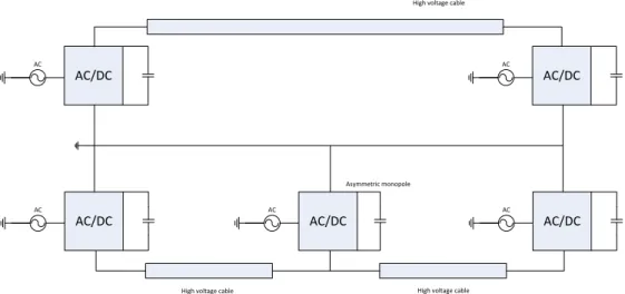
The last point is illustrated in figure 2.7. Connecting monopole converter stations to a larger bipolar system reduce cost and the need for extra space compared to a full bipolar station. This is especially interesting for offshore oil platforms and wind farms, since it is expensive to provide the extra room needed for a second converter when building in the ocean.

(33)

2.4. Converter technologies in an MTDC system 13

AC/DC AC/DC

AC AC

High voltage cable

AC/DC AC/DC AC/DC

AC AC AC

Asymmetric monopole

Figure 2.7: Asymmetric monopole connected to a two converter bipolar sys-tem

2.4 Converter technologies in an MTDC system

2.4.1 Current Source Converters and Voltage Source

Con-verters

As mentioned earlier, a new converter technology was introduced in 1997, known as Voltage Source Converters (VSC), or Self Commutated Converters (SCC). Prior to this, converter stations used in power transmission were so called Current Source Converters (CSC), also known as Line Commutated Converters (LCC). The CSC uses thyristors arranged in a so called Graetz bridge for commutating current from the different phases in an AC system [7]. The layout is illustrated in figure 2.8. The thyristors used in CSCs can be made conducting by applying a control signal, but in order to stop conducting, the AC current must naturally approach zero [11, p. 18]. This means the CSC is reliant on an operating AC grid to turn off its semiconductors. Also, if the charges left in the thyristor after being turned off are not removed properly, a rising voltage at the anode may cause a misfire, potentially short circuiting the DC terminals of the CSC [12]. This is known as a

(34)

AC

DC

Figure 2.8: 6-pulse Current Source Converter - Arrangement of thyristors commutation failure and may occur as a consequence of AC voltage disturbances [1].

A VSC is made up of transistor and diode pairs, arranged in a similar manner to the thyristors of a CSC. The layout is illustrated in figure 2.9. Different transistors can be used, but the most common for power transmission is the Insulated Gate Bipolar Transistor (IGBT). Unlike thyristors, transistors can be turned both on and off by a command signal [11, p.27].

The use of IGBTs gives the VSC several advantages compared to the CSC. Some of the advantages most relevant for an MTDC system are given in [1] and listed below:

• Black start capability of islanded grid

• No chance of commutation failure during AC grid faults • Control of both active and reactive power

• Power direction is changed by reversing current direction rather than

(35)

AC

DC

Figure 2.9: 6-pulse Voltage Source Converter - Arrangement of transistors For these reasons, it is generally accepted that a future MTDC system will have to be based around the VSC. However, while superior to the CSC when considering operational characteristics, the VSC is very vulnerable to DC side short circuit failures [1]. This is primarily due to the filtering DC capacitor and the diodes installed in the Gratz bridge, and will be further explained in the following sections.

2.4.2 VSC configurations

The diodes and IGBTs can be arranged in different ways. The different construc-tions can be divided in two basic groups; based around the classic Graetz bridge design, or as a Modular Multilevel Converter (MMC) [13]. Different variations of both designs are presented in this section.

2.4.2.1 Two-level VSC

The half bridge two-level VSC is the simplest design available. It involves six diode and IGBT pairs arranged in a Graetz bridge, as was shown in figure 2.9 on page 15. In addition to the semiconductors, there is also DC side filter capacitance. In order to increase the voltage blocking capability of the VSC, each valve arm will typically consist of several IGBT/diode pairs connected in series, operating in unison [9].

(36)

Figure 2.10: The full bridge VSC for connection to a single phase. Taken from[18]

AC voltage produced by the half-bridge two-level VSC varies between the voltage levels of either DC terminal. By adding an additional IGBT/diode pair, the full bridge VSC is realised [14, p. 10], depicted in figure 2.10. The full bridge VSC can output AC voltage amplitude twice as large as that of the half bridge VSC, giving a better utilization of the DC voltage and switch cells [14, p. 10].

Since the voltage level can only be varied between two different levels, there is substantial need for filtering [15]. On the DC side, filtering depends on a rather large capacitor which will be discharged during a DC fault, causing large initial fault currents [9, 16]. Also, if a DC fault occurs, there is no way to completely block current through the converter, as the diodes will continue conducting, even after the IGBTs have been blocked [17]. On the other hand, the two-level converter is the simplest VSC available, making it both cheaper to construct and easier to operate than any alternative.

2.4.2.2 Multi level VSC

By connecting extra diodes to the valve arms as illustrated in 2.11, a multilevel VSC is realised. When such a converter is operating as an inverter, the produced AC voltage will have reduced harmonic distortion compared to the two-level VSC. This is because the AC voltage waveform can be made up in several steps rather than just two [19, p.221]. The trade offfor this improved AC voltage is an increase in equipment complexity and cost. In addition, controlling such devices will be more difficult than the simple level VSC [19, p. 219]. Also, as with the two-level VSC, the large DC capacitor and free current path through the diodes makes the design vulnerable to DC faults.

(37)

Figure 2.11: Five-level VSC phase leg. Taken from [19, p. 218] 2.4.2.3 Modular Multilevel Converter

The MMC is made up of several sub modules connected in series, each series connection making up one leg of the converter [13]. The design is illustrated in figure 2.12. There are different sub module designs available, the simplest being the half bridge sub module which is depicted in figure 2.13. Other examples of sub modules are the full-bridge sub module in figure 2.14 and clamp-double sub module in figure 2.15 [20]. The clamped-double sub module is similar to the full-bridge, but the extra diode reduce the number of IGBTs that current must flow through during normal operation, thus reducing on-state losses. All the alternatives have an incorporated capacitance in each sub module. This means there is no need for a separate DC side capacitor for filtering and energy storage [13].

The multi level arrangement of sub modules allows the MMC to access several DC voltage levels when acting as an inverter, giving it the same advantage as the multi level VSC [13]. In addition, since there is no large DC capacitor, the issue of a large initial current transient is removed [13]. Also, if the sub modules used are either full-bridge or clamped-double sub modules, the MMC is capable of completely blocking AC current from flowing into a DC fault [20]. However, these advantages come at the expense of increased complexity, cost and size of the converter [15].

(38)

Figure 2.12: The modular multilevel converter, placement of submodules (SM)

(39)

2.5. Cable design 19

Figure 2.14: The full bridge sub module as proposed in [20]

Figure 2.15: The clamped double sub module as proposed in [20]

2.5 Cable design

Most HVDC cables in use today are so called mass impregnated cables, insulated by oil impregnated paper. An alternative to this is extruded cables, isolated with polymers. Cables insulated with polymers, such as XLPE for example, are generally lighter and less expensive than expensive than the mass impregnated ones. However, polymers are dielectrics, so when exposed to a voltage difference, all the charges in the polymer align. Changing polarity of the voltage can cause electrical trees to form in the insulation, shortening the cable life time and possibly causing DC ground fault [7]. This is a problem when using CSC, as power reversal is done by changing voltage polarity. With the use of VSC, this is no longer an issue, and polymer insulated cables are generally seen as the preferred choice over mass impregnated ones [7].

The cable is constructed in several layers, illustrated in 2.16. The central con-ductor is made of copper or aluminium, and is insulated by a dielectric polymer,

(40)

Figure 2.16: Cable cross section. Figure from the PSCAD library

for example cross linked polyethylene (XLPE). Outside the insulation is a metal sheath, grounded in either end of the cable [21]. Submarine cables will be subjected to a lot of force, especially during installation. Metal wires known as armour are twisted around the cable to protect it against crushing and twisting forces [21]. The sheath and armour is separated by a second layer of polymer. The whole cable is wrapped in a waterproof material. In between each layer there is usually some sort of filler material, in addition to special tape on the interface between in-sulation and metal [21]. Naturally, there will be a potential difference between the conductor and the earthed metal sheath. Since these are separated by a dielectric, the cable essentially becomes a large coaxial capacitor.

2.6 Current interruption in HVDC systems

When current is interrupted by separating two conducting contacts, an arc is formed [22]. In AC systems, this is extinguished by the naturally occurring cur-rent zero crossing, which is a result of the changing curcur-rent and voltage polarity. Current interruption is therefore a lot more difficult in DC systems, since there are no polarity variations [22].

Up until very recently, the only option for clearing faults in HVDC systems has been to activate current breakers in the connected AC systems. For use in MTDC systems, such a method is proposed as the ”handshake method” [23]. This method involves momentarily disconnecting the entire MTDC system from connected AC systems and then clearing the fault before reconnecting. The time for clearing

(41)

2.6. Current interruption in HVDC systems 21

Figure 2.17: The DC circuit breaker designed by ABB. Taken from [26] a fault and restoring grid operation using this method has been reported as 0.5 seconds [23]. If MMCs are used, they can perform current interruption as explained in section 2.4.2.3, which would be much faster than the AC breakers, thus reducing fault clearing time. However, the entire DC grid would still have to be taken momentarily off line.

If the interruption time is to be further reduced and only the faulted part of the grid disconnected, fast acting HVDC breakers must be installed at each line in the MTDC system. Such a breaker would have to incorporate semiconductors for creating an artificial current zero crossing [24], and also be able to withstand fast rising currents and high current levels.

Recent years have seen a large interest in developing a fast and reliable HVDC breaker [1], and in November 2012 ABB announced the release of such a device [25], called a “Proactive hybrid HVDC breaker”. This is described in [26] and the design is depicted in figure 2.17. Fast acting mechanical circuit breakers work together with IGBTs in order to commutate and interrupt large fault currents quickly.

The design can be separated into three different sections. First section is the main DC breaker, comprised of several IGBTs connected in series, each connected in parallel with an arrester. The second section is a bypass made up of a single IGBT and a fast mechanical disconnector. This is connected in parallel with the main breaker. The third section is comprised of a reactor connected in series with a mechanical isolator, which in turn are connected in series with the other two sections. This design allows for fast interruption of large fault currents, while keeping on-state losses at a minimum [26].

(42)

The proposed solution also has the ability of proactive operation. When a fault occurs, the breaker can be put on standby until it is decided whether it need to be opened or not [26]. If the breaker then needs to operate, current will be interrupted within a few µs. While in standby mode, current flows through the IGBTs of the

main breaker, which could operate in a specific way to limit the fault current [26]. In [26], the DC breaker is tested in a setup equivalent to a 320 kV, 2 kA system with fault current rising at a rate of 4.5 kA/ms. Results reported opening times below 2 ms and interruption of currents up to 16 kA.

2.7 Current limiters

Low impedance in DC systems leads to higher fault currents. In order to reduce the currents, current limiters may be installed. These are devices with very low resistance in normal operating circumstances, and which respond to increased current magnitude or frequency with an increased impedance. A few examples of such devices are given below.

2.7.1 Tuned LC circuit

The tuned LC circuit uses a linear inductor connected in series with a parallel con-nection of capacitor and a nonlinear inductor. This is depicted in figure 2.18. The inductors and capacitor are dimensioned such that the capacitance and linear in-ductor cancel each other out during normal operation. During fault, the increased current saturates the nonlinear inductor, limiting voltage across the parallel con-nection. In turn, the tuned LC circuit becomes inductive since contribution from the capacitor is reduced [27]. There is no need for external influence in order to make the device inductive, and it has a very small effect on normal state grid operation. It is also quite cost effective and relies upon familiar technology and devices.

2.7.2 Polymer PTC thermistor

The polymer PTC is a polymer fabricate with embedded conducting particles. During normal state, these particle are in contact with each other, creating a low

(43)

2.7. Current limiters 23

Figure 2.18: The concept of a tuned LC circuit

Figure 2.19: PTC during normal operation and at fault

resistance current path. With increased current and subsequent increased heat development, the polymer expands, causing the particles to lose contact with each other, illustrated in figure 2.19. The current path then becomes more resistive, limiting the current [27]. Such devices have a nonlinear temperature-resistance characteristic, with the resistance quickly increasing once a certain temperature is reached [28]. Seeing how heat development in the device can be calculated by

Q = RI2, it seems clear that the device should be able to quickly limit a rising

fault current. Once the fault current has been extinguished, the polymer contracts, reforming the low ohmic path. Polymer PTC resistors are commercially available today, but not for high voltages [27].

2.7.3 Liquid metal

Liquid metal fault current limiters are made by encapsulating liquid metal and placing it in the current path. This has a relatively low resistance. When sub-jected to a large fault current the metal vapourises due to the increased tempera-ture, increasing resistance of the current path. Once current has been succesfully interrupted, the metal cools back down into its liquid phase [27].

(44)

(45)

Chapter 3

Fault current transients

As mentioned, the VSC is vulnerable to DC side faults. These may occur in different parts of the system, either on the VSC itself, in grid junctions or on the cable.

3.1 Basic physics of fault currents

3.1.1 Resistive system

Figure 3.1 illustrate a simple system with a voltage source U and a load RL connected by a transmission line with resistance Rt. Current in the transmission line and load will be given by Ohm’s law I =U/(RL+Rt). When a short circuit fault appears, it is the equivalent of connecting a fault resistance Rf in parallel with RL and assuming that Rf << RL. As a consequence, system current will rise, as it is now given by I =U/(Rf +Rt). Since faults typically does not occur at the load, Rf will also be somewhat reduced.

Magnitude of the fault current in a transmission line is in other words given by the voltage at feed-in point and total fault path resistance. The latter is the sum of fault resistance and resistanc in the transmission line between feed-in and fault point.

(46)

U

Rt

Rf R

I

Figure 3.1: A simple resistive system with fault

Rt

Rf R

I

Figure 3.2: A capacitive system with fault

3.1.2 Capacitive system

By replacing the voltage source with a capacitor a better understanding of fault currents in a capacitive system can be obtained. This is illustrated in figure 3.2, and is a simplified equivalent of a two-level VSC during fault.

A fault somewhere along the transmission line will trigger a discharge of the ca-pacitor. The voltage producing fault current will then be time dependent, and given by equation (3.1), assuming complete discharge. Current in a capacitor is given by equation 3.2 [29, p. 273].

(47)

3.1. Basic physics of fault currents 27 VC(t) =V0e≠ t · (3.1) IC(t) = C dVC dt =≠ V0 Re ≠t · (3.2)

Here, t is time after initiating discharge, V0 is capacitor voltage at fault inception

and· =RC, withR=Rf+RtandC is size of the capacitor. These equations are plotted with different resistance values in figure 3.3. Discharge time depends on

·, meaning a system with large resistance and/or capacitance will need more time

to fully discharge. Both current and voltage derivatives will be large at beginning of the discharge, then gradually decrease.

0 0.002 0.004 0.006 0.008 0.01 0 50 100 150 200 250 300 350 400 450 Time [s] Voltage [kV] 1 Ohm 2 Ohm 4 Ohm 8 Ohm 16 Ohm (a) Voltage 0 0.002 0.004 0.006 0.008 0.01 0 50 100 150 200 250 300 350 400 450 Time [s] Current [kA] 1 Ohm 2 Ohm 4 Ohm 8 Ohm 16 Ohm (b) Current

Figure 3.3: Discharge voltage and current of RC circuit with varying resistance

3.1.3 Transmission lines

Transmission lines are conductors with a long length. Faults with low fault path impedance in a capacitive system will experience fault currents that vary greatly within a very short time window. Since electromagnetic waves are prohibited from moving faster than the speed of light, c, it becomes necessary to express current and voltage along the transmission line as functions of not only time, but also place [30, p. 2.1]. This can be done by applying the following two equations [31,

(48)

p. 19]. Û ˆx =≠L Î ˆt Î ˆx =≠C Û ˆt (3.3)

Position on the line is denoted by x. Solving the equations in (3.3) reveal the

following voltage and current characteristics;

U(x, t) =Uf(x≠vt) +Ur(x+vt) (3.4) I(x, t) = 1 Zc Uf(x≠vt)≠ 1 Zc Ur(x+vt) (3.5) To get a better understanding of how the electromagnetic waves develop, it is nec-essary to represent the transmission line with a pi-equivalent instead of a single resistance. The pi-equivalent is illustrated in figure 3.4 [30, p. 2.2]. Capacitance to ground has been added as well as inductance of the conductor. Resistance, inductance and capacitance can be calaculated using equations 3.6-3.8. Transmis-sion lines can be modelled reasonably well by series connecting a large number of these equivalents [32], but fault currents can be sufficiently explained by using only one. R= fl A [ /m] (3.6) L= µ0 2filn ry ri [H/m] (3.7) C = 2fiÁ lnry ri [F/m] (3.8)

By looking at this pi-equivalent connected to a VSC filter capacitor, we can as-sume that the majority of the system capacitance is located at the converter, and therefore connected in series with the line resistance and inductance. This makes the system a series connected RLC circuit. Such a circuit is shown in figure 3.5 which is used to derive the basic equations explaining currents and voltage during a fault.

(49)

3.1. Basic physics of fault currents 29 DC Rt Lt Ct/2 Ct/2 _R Figure 3.4: A pi-equivalent

R

L

C

+

-V

0

Figure 3.5: A series RLC circuit

Applying Kirchoffs voltage law gives the following equation for the discharge of the capacitor [29, p. 355]. Ri+Ldi dt + 1 C ⁄ t 0 id·+V0 = 0 (3.9)

By differentiating with respect to t and rearranging the terms, the characteristic

equation for a series RLC circuit is obtained [29, p. 355].

d2i dt2 + R l di dt + i LC = 0 (3.10)

This is a second order differential equation. Its roots are found by the following equation [29, p. 356]:

(50)

di dt1,2 =≠ R 2L± Û (₂R L) 2_≠ 1 LC (3.11)

The response from an RLC circuit to the discharge of its capacitance is said to be either critically, over or under damped. This is decided by whether the roots are real or complex, and also if they are equal or different. Two equal and real roots leads to a critical system, while uneven real roots leads to an overdamped system and complex roots leads to an underdamped system. As can be seen from equation (3.11), this is decided by the difference between the two expressions in the square root. These are now denoted as— and Ê0, where

— = R

2L Ê0 =

1

Ô

LC (3.12)

Damping of the system, basically its ability to dissipate energy in the resistance, is determined by size of—, while Ê0 gives the systems natural frequency [33]. The

damping factor is introduced as the ratio between— and Ê0.

’ = —

2 Ê₀2 =

CR2

4L (3.13)

Criteria for critically, over- or underdamped systems are given in table 3.1 [29, p. 356], expressed by the damping factor.

Table 3.1: Criteria for damping of RLC circuit

’ Damping

1 Critical

>1 Over <1 Under

The different responses are shown in figure 3.6 [34]. Similar to the response from an RC circuit, the current (and voltage) derivative is larger at beginning of discharge before reducing nearing steady state.

(51)

3.1. Basic physics of fault currents 31

Figure 3.6: Natural response of an RLC circuit

3.1.4 Transient waves following fault

A fault to ground at time t = 0 cause a local drop in voltage which triggers a

discharge of the transmission line capacitance, causing a negative voltage wave to travel away from the fault, illustrated in figure 3.7. As the wave proceeds along the line, cable capacitance is discharged into the fault [16]. This voltage wave travels at a given speed, determined by per length inductance and capacitance of the line. In a loss less line (R = 0), wave speed is expressed in equation (3.14)[30,

ch. 2.2].

v = Ô1

LC (3.14)

WhereLandCare inductance and capacitance per length of the transmission line,

given by equations 3.7 and 3.8. Once this wave reaches the end of the line, part of it will be reflected back towards the fault, while the rest is transmitted to the other side of the line interface, illustrated in figure 3.8. How much is reflected and transmitted is determined by the reflection and transmission coefficients. These depend on impedance of the line the wave is travelling on and impedance of the

(52)

Figure 3.7: Wave initialized at ground fault location F

Figure 3.8: Wave reflected at converter station B

component it approaches, and are given by equations (3.15) and (3.16) [30, p. 2.12]. Wave impedance of a transmission line is given by equation (3.17) [30, p. 2.6]. ﬂ= Z2≠Z1 Z1+Z2 (3.15) –= 2Z2 Z1+Z2 = 1 +ﬂ (3.16) Zw = Û L C (3.17)

In figure 3.9, voltage and current are given subscriptsr and f for reverse and

for-ward travelling waves. Reflection and transmission coefficients for both terminals are denoted kA and kB, and are determined by equations (3.15) and (3.16). For a system without losses the magnitude of current and voltage waves will only be reduced when reflected/transmitted. In real life, these waves will be attenuated and distorted due to line resistance, corona and other effects [31, p. 21].

3.1.5 Faults in VSC system

In an HVDC grid with VSCs, the first change the voltage wave will encounter is the converter station. A schematic of the system seen from the travelling waves point of

(53)

Figure 3.9: Lattice diagram showing how waves are reflected between two converters and fault point

view is shown in figure 3.10. It is assumed that the IGBTs will block quickly enough to be considered an open circuit, which is a reasonable assumption according to [6, 16, 17]. The voltage wave then sees a path to ground through the capacitor, connected in parallel to a healthy transmission line with a wave impedance as given by equation 3.17. Impedance of a capacitor is given by ZC = (jÊC)≠1. Total impedance seen by the wave is expressed in (3.18), calculation performed in appendix E.

Zeq=Zw 1 +

jÊZwCconv 1 + (ÊZwCconv)2

(3.18) Where Zw is wave impedance of the healthy line andCconv is the converter capac-itance.

Arrival of the negative voltage wave will trigger the discharge of the converter capacitor in a way similar to what was described earlier. This discharge current will contain both high and low frequency components and is discharged towards the fault. Looking at the pi-equivalent, it is clear that impedance along the fault path as well as impedance to ground is dependent on current frequency. Con-sequently, fault current components with high frequency will experience a large series impedance and relatively small impedances to ground, and opposite for low frequency components [30, p. 2.5]. High frequency components can therefore be expected to reduce faster than low frequency components.

(54)

Zw1

Zw2 C

Figure 3.10: Wave approaching a VSC station with neighbouring line con-nected. Z represent the wave impedance of each transmission line, while C is

the converter capacitance

The discharge current travels along the line similar to the voltage wave, being reflected at the fault point. Assuming a small fault impedance so thatRf << Zw, reflection coefficient ﬂ ƒ ≠1 and an equal and opposite wave is reflected back

towards the converter, where it is reflected once again with the impedance given in (3.18). With the assumption thatZw1 ƒZw2 this impedance will never be greater than the one the wave is already travelling along, and so the reflection coefficient must be negative. Since a negative current wave travelling in one direction is equivalent to a positive wave travelling in the opposite direction, the current at the converter station increases until the wave energy is dissipated in the line resistance and a steady state is reached. Relating to figure 3.3 of the natural response of a series RLC circuit, it is clear that the current should be decreasing over time. Due to the reflections of the current, this is not the case, and a current development at the converter similar to that of an over voltage following a lightning strike can be expected, as is described in [30, p. 3.55] and illustrated in figure 3.11. The voltage on the other will experience little change in value at reflection, as the positive and negative wave cancel each other out.

During discharge of the filter capacitance, there is no current going through the converter [17]. The diodes will start to conduct a current once the capacitors are discharged [17].

Due to stored energy in the cable inductance, the initial magnitude of diode current may be quite large, potentially damaging the diodes [17]. For a system with half bridge VSCs, it is therefore important to interrupt current before the filter capacitor is fully discharged.

(55)

3.1. Basic physics of fault currents 35 I t Converter Fault τ 3τ 5τ I1 I1(ρf(-2ρC)-k1) I1(ρf2(-2ρC)2-k2) I1(ρf3(-2ρC)3-k3)

Figure 3.11: Build up of current at converter shown together with the Lattice diagram over arriving waves. Time for wave to travel from fault to converter is denoted by ·. The factor kn is introduced as a damping variable to illustrate

the attenuation of the wave.

Once the cable inductance has been discharged as well, the fault current is dom-inated by contributions from the connected AC grids [16]. After approximately 300 ms, the fault current approaches a steady state value [6].

The different stages of fault development is illustrated in figure 3.13.

3.1.6 E

ff

ect of multiple converter stations

With additional converters in the system, there are several point where the wave can be reflected at. Transmission of the fault wave at the point must then also be taken into account. A line with two converters and a fault between them is shown in figure 3.14. The fault is closer to converter A than B, meaning capacitance at this station will be discharged first. Since resistance, inductance and capacitance is evenly distributed along the line, this capacitor will see a smaller resistance and inductance, and therefore experience a larger discharge current. The current

(56)

Figure 3.12: Fault current development in MTDC grid for different system topologies. a) Radial grid, b) Lightly meshed grid, c) Ring shaped grid, d)

Densely meshed grid. Taken from [6]

wave reaching the fault point is mostly reflected, but if the fault impedance is sufficiently large, a significant part is transmitted to the other part of the line. It will eventually reach station B where it causes a drop in the current, as it is travelling in the opposite direction of the fault current from the station. The effect is a much more chaotic fault current which will not only rise, but also drop. However, for this to have a measurable effect, the fault impedance must be very high, compared to the wave impedance of the line. Otherwise, the reflection coefficient at fault point will be close to -1, resulting in a near perfect reflection and no transmitted wave.

3.1.7 Properties of cables and overhead lines

The resistance, inductance and capacitance per unit length in a transmission line are given by equations (3.6), (3.7) and (3.8) respectively [35, p. 282][30, p. 2.7]. Where ﬂ is resistivity of the conductor, ry and ri are the outer and inner radius of the insulation, A is cross sectional area of the conductor, µ0 is permeability

of free space, and Á = Á0Ár is the insulation permittivity. The construction of a cable was detailed in section 2.5. An overhead line can be equated to a cable using air as insulation, suspended a certain height over the ground. They have distinct different properties due to this.

As was noted in section 2.5, cables are essentially large coaxial capacitors. The inductance will be low as the relationship between outer and inner radius of the

(57)

(a) Stage 1, filter capacitance is discharged

(b) Stage 2, cable discharged through diodes

(c)Stage3, The fault is fed by adja-cent AC grid through diode bridge

Figure 3.13: The three stages of fault development

AC AC

A

B

(58)

insulation is relatively small. The opposite is true for overhead lines, where the large distance to ground gives a large inductance, and in combination with the low permittivity of air (Á ƒ1) a comparably small capacitance [30, p. 2.9]. Some

implications from this are listed below:

• Travelling wave velocity in overhead lines are equal to light speed, while

velocity in cables are lower [30, p. 2.8]

• Fault impedance is lower in cables

• Increased capacitance and lowered inductance gives a higher damping

coef-ficient

3.2 Di

ff

erent kinds of faults

In a bipolar system, fault can occur on either of the poles, causing a monopolar fault, or there can be a short circuit between the poles which will lead to a bipolar fault. Faults are more likely to occur along the line rather than in converters or grid junctions [36]. This is also true for cable based systems, where faults can be caused by degradation of insulation or external damage to the cable. In either case, cable faults are always permanent. While bipolar faults are more severe than monopolar faults , they are unlikely in offshore cable systems since the cables are situated relatively far apart. This greatly reduce the risk of simultaneous damage to both cables [16]. For the purpose of describing fault propagation, the monopolar cable fault will therefore be used as an example in the following sections.

3.3 Parameters that influence the fault current

Magnitude of the current during the initial discharge of filter capacitors are mainly decided by the filter and line capacitance and the total impedance between mea-suring point and fault [16, 32]. The latter is the sum of fault and cable impedance. Reducing the system capacitance will reduce peak value of fault current during the initial phase, and will also shorten discharge time due to the decreased system time constant (· =RCf ilter) [16, 32]. Increased fault impedance and distance will reduce peak fault current and increase discharge time [16, 32].

(59)

3.4. Requirements to fault protection system 39 Once the system enter the freewheeling diodes phase, current is caused by the demagnetising of cable inductance and so the fault current will depend on pre-fault current in the cable and short circuit ratio between the DC grid and connected AC grids [32].

During the final stage when the fault current reaches a steady state, its value is depended upon the fault location, impedance and the Short Circuit Ratio (SCR) between the AC and DC systems [16, 32].

In addition to these, the topology of the grid also matter [6]. A more complex DC grid with several junctions and high mesh grade will experience higher fault currents and faster spread of the fault than a simpler system [6].

3.4 Requirements to fault protection system

A modern protection system consists of three main sub systems [37]. First are the relays, where inputs from current transformers are used to monitor the grid and determine if a fault has occurred. Secondly, a communication system is necessary in order to communicate between the relays, possible central decision making units and the system breakers. The third and final system is made up of the devices re-sponsible for interrupting current. In AC grids this is done by mechanical breakers [22]. The proposed methods for clearing faults in an HVDC grid was presented in sections 2.6 and 2.4.2.3. The following is required of a modern protection system, both in AC and DC grids [5].

• SpeedFast action is important to prevent the fault from spreading to other

parts of the system

• Sensitivity The system must detect all faults, and at the same time not

trigger during normal operation transients

• SelectivityThe system must be able to correctly locate the faulted

compo-nent, and isolate it from the healthy grid

• SeamlessAfter fault clearance, the rest of the power system should be able

(60)

Figure 3.15: The process from detecting fault to normal operation is resumed

• Robustness In