Open Access
Research article
Recursive gene selection based on maximum margin criterion: a
comparison with SVM-RFE
Satoshi Niijima*
1and Satoru Kuhara
2Address: 1Department of Bioinformatics, Graduate School of Systems Life Sciences, Kyushu University, Hakozaki 6-10-1, Higashi-ku, Fukuoka 812-8581, Japan and 2Faculty of Agriculture, Kyushu University, Hakozaki 6-10-1, Higashi-ku, Fukuoka 812-8581, Japan
Email: Satoshi Niijima* - [email protected]; Satoru Kuhara - [email protected] * Corresponding author
Abstract
Background: In class prediction problems using microarray data, gene selection is essential to improve the prediction accuracy and to identify potential marker genes for a disease. Among numerous existing methods for gene selection, support vector machine-based recursive feature elimination (SVM-RFE) has become one of the leading methods and is being widely used. The SVM-based approach performs gene selection using the weight vector of the hyperplane constructed by the samples on the margin. However, the performance can be easily affected by noise and outliers, when it is applied to noisy, small sample size microarray data.
Results: In this paper, we propose a recursive gene selection method using the discriminant vector of the maximum margin criterion (MMC), which is a variant of classical linear discriminant analysis (LDA). To overcome the computational drawback of classical LDA and the problem of high dimensionality, we present efficient and stable algorithms for MMC-based RFE (MMC-RFE). The MMC-RFE algorithms naturally extend to multi-class cases. The performance of MMC-RFE was extensively compared with that of SVM-RFE using nine cancer microarray datasets, including four multi-class datasets.
Conclusion: Our extensive comparison has demonstrated that for binary-class datasets MMC-RFE tends to show intermediate performance between hard-margin SVM-MMC-RFE and SVM-MMC-RFE with a properly chosen soft-margin parameter. Notably, MMC-RFE achieves significantly better performance with a smaller number of genes than SVM-RFE for multi-class datasets. The results suggest that MMC-RFE is less sensitive to noise and outliers due to the use of average margin, and thus may be useful for biomarker discovery from noisy data.
Background
Microarray technology allows us to measure the expres-sion levels of thousands of genes simultaneously. A vast amount of data produced by microarrays pose a great challenge on conventional data mining and machine learning methods, because the number of genes often
exceeds tens of thousands, whereas the number of sam-ples is at most a few hundred.
Along with clustering and classification of genes and/or samples, gene selection is an important aspect of microar-ray data analysis, and has been a central issue in recent Published: 25 December 2006
BMC Bioinformatics 2006, 7:543 doi:10.1186/1471-2105-7-543
Received: 27 July 2006 Accepted: 25 December 2006 This article is available from: http://www.biomedcentral.com/1471-2105/7/543
© 2006 Niijima and Kuhara; licensee BioMed Central Ltd.
This is an Open Access article distributed under the terms of the Creative Commons Attribution License (http://creativecommons.org/licenses/by/2.0), which permits unrestricted use, distribution, and reproduction in any medium, provided the original work is properly cited.
Page 2 of 18 years [1,2]. Specifically, gene selection is used to identify
genes most relevant to sample classification, for example, those differentiate between normal and cancerous tissue samples. Gene selection plays essential roles in classifica-tion tasks. It improves the predicclassifica-tion accuracy of classifi-ers by using only discriminative genes. It also saves computational costs by reducing dimensionality. More importantly, if it is possible to identify a small subset of biologically relevant genes, it may provide insights into understanding the underlying mechanism of a specific biological phenomenon. Also, such information can be useful for designing less expensive experiments by target-ing only a handful of genes.
The most common gene selection approach is so-called gene ranking. It is a univariate approach in the sense that each gene is evaluated individually with respect to a cer-tain criterion that represents class discrimination ability. The criteria often used are e.g., t-statistics, the signal-to-noise (S2N) ratio [3,4] and the between-group to within-group (BW) ratio [5]. Although such gene ranking criteria are simple to use, they ignore correlations or interactions among genes, which may be essential to class discrimina-tion and characterizadiscrimina-tion.
Among existing gene selection methods, support vector machine-based recursive feature elimination (SVM-RFE) [6] has become one of the leading methods and is being widely used. It is a multivariate approach, hence the cor-relations among genes can be taken into account. Moreo-ver, since the selection is based on an SVM classifier, a subset of genes that yields high classification performance can be identified. Recently, the successful application of RFE has motivated the development of several SVM-based gene selection methods [7-9]. The SVM-SVM-based approach performs gene selection using the weight vector of the hyperplane constructed by the samples on the mar-gin, i.e. support vectors. However, while this property may be crucial for achieving good generalization performance, the effect of using support vectors on gene selection remains unclear, especially when it is applied to noisy, small sample size microarray data. A recent work by Li and Yang [10] implies that only penalizing redundant genes for the samples on the margin may lead to poorer per-formance.
In this paper, we propose a recursive gene selection method based on the maximum margin criterion (MMC) [11], which is a variant of classical linear discriminant analysis (LDA). Guyon et al. [6] compared the perform-ance between SVM-RFE and classical LDA-based RFE (LDA-RFE), and claimed that the use of support vectors is critical in eliminating irrelevant genes. However, the com-parison is insufficient in the following respects:
• For computational reasons, LDA-RFE was performed by eliminating half of genes at each iteration, whereas SVM-RFE by eliminating one gene at a time.
• Cross-validation was performed improperly [12]. • The comparison was made only on a single dataset. The computational drawback of classical LDA limits the use of LDA-RFE for gene selection. This paper presents efficient and stable algorithms for MMC-based RFE (MMC-RFE), which overcomes the singularity problem of classical LDA and the problem of high dimensionality. To validate the effectiveness of MMC-RFE, we extensively compare its performance with that of SVM-RFE using nine cancer microarray datasets.
Results and discussion
Datasets
In this study, we used nine public datasets of cancer microarrays. Five of the datasets concern binary-class pre-diction problems: normal versus tumor for Colon cancer [13] and Prostate cancer [14], ALL versus AML for Leuke-mia [3], and clinical outcome for Medulloblastoma [15] and Breast cancer [16]. Four of the datasets are on multi-class subtype prediction problems: MLL [17], SRBCT [18], CNS [15], and NCI60 [19]. The details of these datasets are described below:
Colon cancer dataset [13]
This Affymetrix high-density oligonucleotide array dataset contains 62 samples from 2 classes of colon-cancer patients: 40 normal healthy samples and 22 tumor sam-ples. The expression profiles of 2000 genes are used. The dataset is publicly available at [20].
Prostate cancer dataset [14]
This Affymetrix high-density oligonucleotide array dataset contains 102 samples from 2 classes: 50 normal tissue samples and 52 prostate tumor samples. The expression profiles of 12600 genes are used. The dataset is publicly available at [21].
Leukemia dataset [3]
This Affymetrix high-density oligonucleotide array dataset contains 38 samples from 2 classes of leukemia: 27 acute lymphoblastic leukemia (ALL) and 11 acute myeloid leukemia (AML). The expression profiles of 7129 genes are used. The dataset is publicly available at [21]. Other 34 samples consisting of 20 ALL and 14 AML are used as an independent test set as mentioned later.
Medulloblastoma dataset [15]
This Affymetrix high-density oligonucleotide array dataset contains 60 samples from 2 classes on patient survival
with medulloblastoma: 21 treatment failures and 39 sur-vivors. The expression profiles of 7129 genes are used. The dataset is publicly available at [21].
Breast cancer dataset [16]
This cDNA microarray dataset contains 76 samples from 2 classes on five-year metastasis-free survival: 33 poor prog-nosis and 43 good progprog-nosis. The expression profiles of 4918 genes are used. The dataset is publicly available at [22]. Other 19 samples with 12 poor prognosis and 7 good prognosis are used as an independent test set as mentioned later.
MLL dataset [17]
This Affymetrix high-density oligonucleotide array dataset contains 57 samples from 3 classes of leukemia: 20 acute lymphoblastic leukemia (ALL), 17 mixed-lineage leuke-mia (MLL), 20 acute myelogenous leukeleuke-mia (AML). The expression profiles of 12582 genes are used. The dataset is publicly available at [21]. Note that a test dataset consist-ing of 15 samples is not used here.
SRBCT dataset [18]
This cDNA microarray dataset contains 63 samples from 4 classes of small round blue-cell tumors of childhood (SRBCT): 23 Ewing family of tumors, 20 rhabdomyosar-coma, 12 neuroblastoma, and 8 non-Hodgkin lym-phoma. The expression profiles of 2308 genes are used. The dataset is publicly available at [23]. Note that a test dataset consisting of 20 SRBCT and 5 non-SRBCT samples is also available, but is not used here.
CNS dataset [15]
This Affymetrix high-density oligonucleotide array dataset contains 42 samples from 5 different tumors of the central nervous system (CNS): 10 medulloblastomas, 10 malig-nant gliomas, 10 atypical teratoid/rhabdoid tumors, 8 primitive neuro-ectodermal tumors, and 4 human cere-bella. The expression profiles of 7129 genes are used. The dataset is publicly available at [21].
NCI60 dataset [19]
This cDNA microarray dataset contains 61 samples from 8 classes of human tumor cell lines: 9 breast, 5 CNS, 7 colon, 8 leukemia, 8 melanoma, 9 non-small cell lung car-cinoma, 6 ovarian, and 9 renal tumors. The expression profiles of 3938 genes are used. The dataset is publicly available at [24].
Preprocessing
For the Prostate cancer, Leukemia, Medulloblastoma, MLL, and CNS datasets, expression values were first thresholded with a floor of 100 (10 for Prostate cancer) and a ceiling of 16000, followed by a base 10 logarithmic transform. Then, each sample was standardized to zero
mean and unit variance across genes. For the Colon cancer dataset, after a base 10 logarithmic transform, each sam-ple was standardized. For the Breast cancer dataset, after the filtering of genes following [16], each sample was standardized. For the NCI60 dataset, after filtering genes with missing values, a base 2 logarithmic transform and standardization were applied. For the SRBCT dataset, the expression profiles already preprocessed following [18] were used.
Gene selection methods for comparison
As a baseline gene selection criterion, we employed the S2N ratio [4] for binary-class problems, and the BW ratio [5] for multi-class problems. Top-ranked genes with the largest ratios were used for classification. We primarily compared two algorithms for MMC-RFE, called uncorre-lated MMC-RFE and orthogonal MMC-RFE (see Meth-ods), with SVM-RFE. For the SVM classifier, we used both hard-margin SVM and soft-margin SVM with linear ker-nel. The effect of using support vectors on gene selection may be directly evaluated by hard-margin SVM, i.e. when setting the soft-margin parameter C to infinity. The use of soft-margin SVM can alleviate the influence of noise and outliers to some extent and avoid overfitting of the data, with the trade-off between training errors and the margin. In the experiments, we used a wide range of values for the C parameter: C = {0.001, 0.01, 0.1, 1, 10, 100, 1000}. The extension of SVM to more than two classes is not obvious. Hence, several approaches have been proposed for multi-class SVMs, of which we employed one-versus-all SVM (OVASVM). Ramaswamy et al. [25] showed the effective-ness of the OVASVM approach for gene selection and clas-sification, and Weston et al. [8] also applied it to gene selection in multi-class problems. In this study, OVASVM-based RFE was performed in the same way as in [8]. For the implementation of SVM-RFE, we exploited the Spider library for MATLAB, which is publicly available from [26].
Performance evaluation
We assessed the performance of each gene selection method by repeated random splitting; the samples were partitioned randomly in a class proportional manner into a training set consisting of two-thirds of the whole sam-ples and a test set consisting of the held-out one-third of the samples. To avoid selection bias, gene selection was performed using only the training set, and the classifica-tion error rate of the learnt classifier was obtained using the test set. This splitting was repeated 100 times. The error rates averaged over the 100 trials and the corre-sponding standard error rates are reported.
As a baseline classification method, we employed the nearest mean classifier (NMC), which has been found effective for cancer classification [27]. We combined each gene selection method with NMC. Although the nearest
Page 4 of 18 neighbor classifier (NNC) was applied as well, NMC
con-sistently showed favorable performance compared with NNC in the repeated random splitting experiments, and thus the results on NMC are reported here. While the per-formances of the gene selection methods can be com-pared fair by using the same classifier, SVM-RFE is often used as an integrated method of gene selection and classi-fication, and MMC-RFE may also perform better when used with the MMC classifier (see Methods). With this view, we further compared the performance between SVM-RFE in combination with the SVM classifier and MMC-RFE with the MMC classifier. For multi-class data-sets, the OVASVM classifier was used.
As suggested by Weston et al. [8], to save computational time of RFE, we removed half of the genes until less than 1000, and then a single gene at a time. In this study, we do not address the problem of finding the optimum number of genes that would yield highest classification accuracy. Instead, the number of genes was varied from 1 to 100, and the performances were compared for each number of genes.
Performance comparison for binary-class datasets
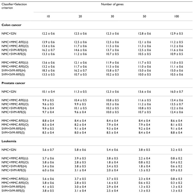
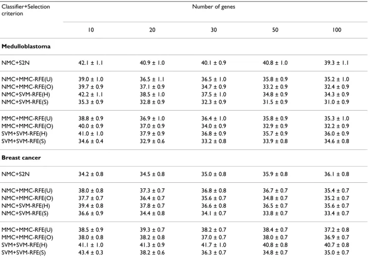
Tables 1 and 2 show the average error and standard error rates of each combination of classifiers and gene selection criteria for the binary-class datasets: Colon cancer, Pros-tate cancer, Leukemia, Medulloblastoma, and Breast can-cer. Figures 1 and 2 plot the average error rates as a function of the number of genes from 1 to 100. In the tables and figures, MMC-RFE(U), MMC-RFE(O), SVM-RFE(H) and SVM-RFE(S) stand for uncorrelated MMC-RFE, orthogonal MMC-MMC-RFE, hard-margin SVM-RFE and soft-margin SVM-RFE, respectively. For SVM-RFE(S), the best result with respect to the C parameter is shown. Our observations from these results are as follows:
• NMC+MMC-RFE(U,O) versus NMC+SVM-RFE(H,S) – Overall, MMC-RFE(U,O) shows intermediate perform-ance between SVM-RFE(H) and SVM-RFE(S) with the best C parameter. MMC-RFE(O) is consistently better than MMC-RFE(U), and notably MMC-RFE(O) performs the best for Leukemia. In most cases, however, the difference is not significant and they are quite competitive.
• MMC+MMC-RFE(U,O) versus SVM+SVM-RFE(H,S) – The performance of MMC-RFE(U,O) is improved for Pros-tate cancer. For the other datasets, the trend is similar to the case of using NMC.
• S2N versus MMC-RFE(U,O), SVM-RFE(H,S) – Both MMC-RFE(U,O) and SVM-RFE(H,S) improve the per-formance of NMC over S2N for Prostate cancer, Leukemia and Medulloblastoma. Wessels et al. [27] have reported that NMC with S2N performs the best among various
combinations of gene selection methods and classifiers for Colon cancer and Breast cancer. Consistently with their results, S2N performs better than SVM-RFE(H) for these datasets. However, a significant improvement is achieved for SVM-RFE(S) by setting the C parameter to a small value, e.g. 0.001. Huang and Kecman [28] also reported that the finer tuning of the C parameter can sig-nificantly improve the performance of SVM-RFE.
Guyon et al. [6] have drawn a conclusion from their result on the Colon cancer dataset that SVM-RFE performs better than both S2N and LDA-RFE. In their experiment, the C parameter was set to 100. However, SVM-RFE(S) with C = 100 gives almost the same error rate as SVM-RFE(H) for all the binary-class datasets in our study, and its performance is poorer than that of S2N for Colon cancer, as mentioned previously. There are some reasons that account for this contradiction. First, although Guyon et al. [6] used SVM and weighted voting [3] for classification, we have found that for the Colon cancer dataset, SVM with C = 100 per-forms significantly worse than NMC when combined with S2N. As can be seen from Table 1, NMC+SVM-RFE(H) performs even favorably against SVM+SVM-RFE(H). Sec-ond, this can be attributed to the selection bias caused by their improper use of cross-validation [12]; they failed to include the gene selection process in the cross-validation. Finally, the performance difference between LDA-RFE and SVM-RFE may be due to the difference in the number of genes eliminated at a time.
Guyon et al. [6] also compared the performance between the mean squared error-based RFE (MSE-RFE) and SVM-RFE, and claimed the superiority of SVM-RFE. However, our results suggest that MSE-RFE might also show better performance in some cases. Indeed, this has been implied by the work of Li and Yang [10], which showed that ridge regression-based RFE performed better than SVM-RFE. It should be noted that MSE is closely related to classical LDA and ridge regression [29,30]. MMC-RFE is still advan-tageous over LDA-RFE and MSE-RFE, because MMC-RFE does not need to compute the inverse of a matrix, which makes MMC-RFE a computationally efficient and stable method.
As our results indicate, the prediction of clinical outcome is generally more difficult than that of tissue or disease types. The error rates of NMC with S2N for the clinical outcome datasets (Medulloblastoma and Breast Cancer) almost coincide with the results presented in [31], which performed a comparative study on outcome prediction using the same validation strategy as our study. The result for Medulloblastoma shows that the prediction perform-ance can be improved by multivariate gene selection methods such as MMC-RFE and SVM-RFE. However, it is
Table 1: Performance comparison for binary-class datasets. Classifier+Selection criterion Number of genes 10 20 30 50 100 Colon cancer NMC+S2N 12.2 ± 0.6 12.5 ± 0.6 12.3 ± 0.6 12.8 ± 0.6 12.9 ± 0.5 NMC+MMC-RFE(U) 13.9 ± 0.6 12.5 ± 0.6 12.5 ± 0.6 12.1 ± 0.6 11.2 ± 0.5 NMC+MMC-RFE(O) 13.4 ± 0.6 11.7 ± 0.6 11.5 ± 0.6 11.3 ± 0.6 11.2 ± 0.6 NMC+SVM-RFE(H) 16.2 ± 0.7 14.6 ± 0.6 13.7 ± 0.6 12.5 ± 0.6 11.6 ± 0.6 NMC+SVM-RFE(S) 13.3 ± 0.6 11.2 ± 0.6 10.7 ± 0.5 10.5 ± 0.5 10.9 ± 0.5 MMC+MMC-RFE(U) 13.6 ± 0.6 12.1 ± 0.6 11.9 ± 0.6 11.7 ± 0.5 11.0 ± 0.5 MMC+MMC-RFE(O) 13.2 ± 0.6 11.7 ± 0.6 11.5 ± 0.6 11.0 ± 0.6 11.1 ± 0.6 SVM+SVM-RFE(H) 18.3 ± 0.6 16.2 ± 0.7 15.8 ± 0.7 15.0 ± 0.6 15.0 ± 0.6 SVM+SVM-RFE(S) 13.5 ± 0.5 10.7 ± 0.5 10.2 ± 0.5 10.0 ± 0.5 10.5 ± 0.6 Prostate cancer NMC+S2N 10.1 ± 0.4 11.3 ± 0.5 12.3 ± 0.6 13.6 ± 0.6 16.0 ± 0.7 NMC+MMC-RFE(U) 9.9 ± 0.5 10.4 ± 0.5 10.8 ± 0.5 11.6 ± 0.5 13.4 ± 0.6 NMC+MMC-RFE(O) 9.6 ± 0.5 9.9 ± 0.5 10.3 ± 0.6 11.2 ± 0.6 13.5 ± 0.7 NMC+SVM-RFE(H) 9.6 ± 0.4 10.1 ± 0.5 10.2 ± 0.5 10.8 ± 0.5 12.2 ± 0.6 NMC+SVM-RFE(S) 9.7 ± 0.4 9.6 ± 0.4 10.0 ± 0.5 10.7 ± 0.5 12.4 ± 0.6 MMC+MMC-RFE(U) 8.8 ± 0.4 8.4 ± 0.4 8.4 ± 0.4 8.4 ± 0.4 8.6 ± 0.4 MMC+MMC-RFE(O) 8.5 ± 0.4 8.2 ± 0.4 7.9 ± 0.4 7.9 ± 0.4 8.1 ± 0.5 SVM+SVM-RFE(H) 9.9 ± 0.5 9.1 ± 0.4 9.3 ± 0.4 9.2 ± 0.4 9.1 ± 0.4 SVM+SVM-RFE(S) 8.5 ± 0.4 8.0 ± 0.4 8.5 ± 0.4 8.4 ± 0.4 8.8 ± 0.4 Leukemia NMC+S2N 5.6 ± 0.7 5.8 ± 0.6 5.4 ± 0.6 3.8 ± 0.5 3.2 ± 0.5 NMC+MMC-RFE(U) 5.7 ± 0.6 3.9 ± 0.5 3.8 ± 0.5 2.2 ± 0.4 0.8 ± 0.2 NMC+MMC-RFE(O) 5.8 ± 0.6 2.8 ± 0.5 1.8 ± 0.4 0.8 ± 0.2 0.4 ± 0.2 NMC+SVM-RFE(H) 5.4 ± 0.6 3.8 ± 0.5 3.4 ± 0.5 1.8 ± 0.4 0.6 ± 0.2 NMC+SVM-RFE(S) 6.0 ± 0.6 3.1 ± 0.4 2.0 ± 0.4 1.5 ± 0.3 0.9 ± 0.3 MMC+MMC-RFE(U) 5.6 ± 0.6 3.7 ± 0.5 3.7 ± 0.5 2.3 ± 0.4 0.8 ± 0.3 MMC+MMC-RFE(O) 5.8 ± 0.6 2.8 ± 0.5 1.6 ± 0.3 0.6 ± 0.2 0.3 ± 0.2 SVM+SVM-RFE(H) 4.1 ± 0.5 3.0 ± 0.4 2.9 ± 0.4 1.3 ± 0.3 1.3 ± 0.3 SVM+SVM-RFE(S) 3.8 ± 0.5 3.1 ± 0.4 2.5 ± 0.4 1.3 ± 0.3 1.3 ± 0.3 The average error and standard error rates (%) for Colon cancer, Prostate cancer and Leukemia, when the number of genes is {10, 20, 30, 50, 100}. SVM-RFE(S) shows the best result with respect to the C parameter; NMC+SVM-RFE(S): C = 0.01, SVM+SVM-RFE(S): C = 0.01 for Colon cancer; NMC+SVM-RFE(S): C = 0.01, SVM+SVM-RFE(S): C = 0.01 for Prostate cancer; NMC+SVM-RFE(S): C = 0.001, SVM+SVM-RFE(S): C = 100 for Leukemia.
Page 6 of 18 at best an error rate of above 30% on average, when using
two-thirds of the samples as a training set.
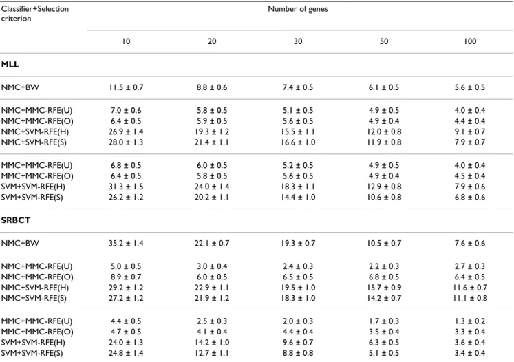
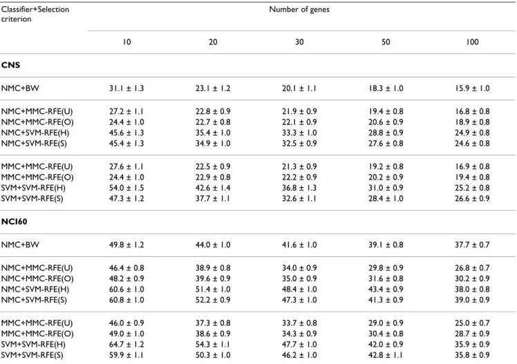
Performance comparison for multi-class datasets
Tables 3 and 4 show the average error and standard error rates of each combination of classifiers and gene selection criteria for the multi-class datasets: MLL, SRBCT, CNS and NCI60. Figures 3 and 4 plot the average error rates as a function of the number of genes from 1 to 100. The OVASVM approach was used here for SVM-RFE. We observe from these results the following:
• NMC+MMC-RFE(U,O) versus NMC+SVM-RFE(H,S) – MMC-RFE(U,O) outperforms SVM-RFE(H,S) for all the datasets; it shows significantly better performance for a smaller number of genes. MMC-RFE(U) appears to be bet-ter than MMC-RFE(O) for SRBCT, while they are compa-rable for the other datasets.
• MMC+MMC-RFE(U,O) versus SVM+SVM-RFE(H,S) – The trend is similar to the case of using NMC. Although the performance of NMC+SVM-RFE(H,S) is improved by
SVM+SVM-RFE(H,S) for SRBCT, it is still outperformed by both NMC+MMC-RFE(U,O) and MMC+MMC-RFE(U,O). • BW versus RFE(U,O), SVM-RFE(H,S) – MMC-RFE(U,O) shows better performance than BW for three datasets (MLL, SRBCT and NCI60), while performs com-petitively with BW for CNS. In contrast, SVM-RFE(H,S) performs even worse than BW for these datasets, which suggests that OVASVM may not be suitable for selecting a small number of discriminative genes.
Taken together, our extensive comparison has demon-strated that for binary-class datasets MMC-RFE tends to show intermediate performance between hard-margin SVM-RFE and SVM-RFE with a properly chosen C param-eter. Notably, MMC-RFE achieves significantly better per-formance with a smaller number of genes than SVM-RFE for multi-class datasets.
The results on hard-margin SVM-RFE indicate that the use of support vectors is not necessarily effective for achieving better performance in gene selection. Because the SVM-Table 2: Performance comparison for binary-class datasets (continued).
Classifier+Selection criterion Number of genes 10 20 30 50 100 Medulloblastoma NMC+S2N 42.1 ± 1.1 40.9 ± 1.0 40.1 ± 0.9 40.8 ± 1.0 39.3 ± 1.1 NMC+MMC-RFE(U) 39.0 ± 1.0 36.5 ± 1.1 36.5 ± 1.0 35.8 ± 0.9 35.2 ± 1.0 NMC+MMC-RFE(O) 39.7 ± 0.9 37.1 ± 0.9 34.7 ± 0.9 33.2 ± 0.9 32.4 ± 0.9 NMC+SVM-RFE(H) 42.2 ± 1.1 38.5 ± 1.0 37.5 ± 1.0 34.8 ± 0.9 34.3 ± 0.9 NMC+SVM-RFE(S) 35.3 ± 0.9 32.8 ± 0.9 32.3 ± 0.9 31.5 ± 0.9 31.0 ± 0.9 MMC+MMC-RFE(U) 38.8 ± 0.9 36.9 ± 1.0 36.4 ± 1.0 35.8 ± 0.9 35.3 ± 1.0 MMC+MMC-RFE(O) 40.0 ± 0.9 37.0 ± 0.9 34.0 ± 0.9 32.9 ± 0.9 32.2 ± 0.9 SVM+SVM-RFE(H) 41.0 ± 1.0 37.9 ± 0.9 36.8 ± 0.9 35.7 ± 0.9 36.0 ± 0.9 SVM+SVM-RFE(S) 34.6 ± 0.4 32.9 ± 0.6 33.2 ± 0.8 33.9 ± 0.8 34.6 ± 0.8 Breast cancer NMC+S2N 34.2 ± 0.8 34.5 ± 0.8 35.0 ± 0.8 35.9 ± 0.8 36.1 ± 0.8 NMC+MMC-RFE(U) 38.0 ± 0.8 37.3 ± 0.7 36.8 ± 0.8 36.7 ± 0.7 35.4 ± 0.7 NMC+MMC-RFE(O) 37.7 ± 0.7 36.4 ± 0.7 35.6 ± 0.7 34.8 ± 0.7 35.2 ± 0.7 NMC+SVM-RFE(H) 39.4 ± 0.8 37.8 ± 0.7 36.6 ± 0.8 36.5 ± 0.7 35.6 ± 0.7 NMC+SVM-RFE(S) 36.6 ± 0.9 34.4 ± 0.8 34.1 ± 0.7 33.8 ± 0.7 33.4 ± 0.7 MMC+MMC-RFE(U) 38.5 ± 0.9 39.3 ± 0.7 38.2 ± 0.7 38.4 ± 0.7 37.2 ± 0.8 MMC+MMC-RFE(O) 38.0 ± 0.8 38.2 ± 0.8 37.0 ± 0.7 38.0 ± 0.7 36.9 ± 0.7 SVM+SVM-RFE(H) 41.1 ± 1.0 41.3 ± 0.9 41.7 ± 1.0 40.8 ± 0.8 40.7 ± 0.8 SVM+SVM-RFE(S) 43.4 ± 0.3 38.2 ± 0.6 36.3 ± 0.7 34.8 ± 0.7 35.0 ± 0.7 The average error and standard error rates (%) for Medulloblastoma and Breast cancer, when the number of genes is {10, 20, 30, 50, 100}. SVM-RFE(S) shows the best result with respect to the C parameter; NMC+SVM-RFE(S): C = 0.001, SVM+SVM-RFE(S): C = 0.01 for Medulloblastoma; NMC+SVM-RFE(S): C = 0.001, SVM+SVM-RFE(S): C = 0.001 for Breast cancer.
based approach to gene selection uses the weight vector of the hyperplane constructed by the training samples clos-est to the decision boundary, the performance can be eas-ily affected by noise and possible outliers. As the results on the binary-class datasets show, SVM-RFE can achieve a significant improvement for some of the datasets by set-ting the C parameter to a small value. The soft-margin parameter plays more roles than just handling noisy data; it is effective for linearly inseparable cases and crucial for avoiding overfitting.
In contrast, MMC-RFE uses the discriminant vector obtained by maximizing the average margin, hence less sensitive to noise and outliers. In addition, no parameters need to be tuned. Although MMC-RFE may not be so flex-ible as soft-margin SVM-RFE, orthogonal MMC-RFE shows comparable performance to SVM-RFE with the best C parameter for some cases. Another advantage of MMC-RFE is that it naturally extends to multi-class cases, while
the SVM-based approach typically treats them by decom-posing the multi-class problems into many binary-class ones, e.g. one-versus-one and one-versus-all strategies. Therefore, MMC-RFE is in particular effective for gene selection in multi-class problems, which has also been validated by the performance on the multi-class datasets.
Comparison of selected genes
It is clearly of interest to compare the selected genes of MMC-RFE with those of S2N and SVM-RFE. To this end, we conducted additional experiments using independent test sets. The results were obtained for the Prostate cancer, Leukemia, and Breast cancer datasets. Note that the test set for Prostate cancer is from [32], which is available at [33]. It contains 25 normal tissue samples and 9 prostate tumor samples. Gene selection was performed using the whole samples in the previous experiment, and the classification error rate of the learnt classifier was obtained using the independent test set. NNC and NMC were used here for Performance comparison for binary-class datasets
Figure 1
Performance comparison for binary-class datasets. The average error rates (%) as a function of the number of genes from 1 to 100, for Colon cancer, Prostate cancer and Leukemia.
0 20 40 60 80 100 0 5 10 15 20 25 30 35 Number of genes Error rate (%) Colon cancer NMC+S2N NMC+MMC−RFE(U) NMC+MMC−RFE(O) NMC+SVM−RFE(H) NMC+SVM−RFE(S) 0 20 40 60 80 100 0 5 10 15 20 Number of genes Error rate (%) Prostate cancer NMC+S2N NMC+MMC−RFE(U) NMC+MMC−RFE(O) NMC+SVM−RFE(H) NMC+SVM−RFE(S) 0 20 40 60 80 100 0 5 10 15 20 Number of genes Error rate (%) Leukemia NMC+S2N NMC+MMC−RFE(U) NMC+MMC−RFE(O) NMC+SVM−RFE(H) NMC+SVM−RFE(S) 0 20 40 60 80 100 0 5 10 15 20 25 30 35 Number of genes Error rate (%) Colon cancer MMC+MMC−RFE(U) MMC+MMC−RFE(O) SVM+SVM−RFE(H) SVM+SVM−RFE(S) 0 20 40 60 80 100 0 5 10 15 20 Number of genes Error rate (%) Prostate cancer MMC+MMC−RFE(U) MMC+MMC−RFE(O) SVM+SVM−RFE(H) SVM+SVM−RFE(S) 0 20 40 60 80 100 0 5 10 15 20 Number of genes Error rate (%) Leukemia MMC+MMC−RFE(U) MMC+MMC−RFE(O) SVM+SVM−RFE(H) SVM+SVM−RFE(S)
Page 8 of 18 Performance comparison for binary-class datasets (continued)
Figure 2
Performance comparison for binary-class datasets (continued). The average error rates (%) as a function of the number of genes from 1 to 100, for Medulloblastoma and Breast cancer.
0 20 40 60 80 100 0 5 10 15 20 25 30 35 40 45 50 Number of genes Error rate (%)
Medulloblastoma
NMC+S2N NMC+MMC−RFE(U) NMC+MMC−RFE(O) NMC+SVM−RFE(H) NMC+SVM−RFE(S) 0 20 40 60 80 100 0 5 10 15 20 25 30 35 40 45 50 Number of genes Error rate (%)Breast cancer
NMC+S2N NMC+MMC−RFE(U) NMC+MMC−RFE(O) NMC+SVM−RFE(H) NMC+SVM−RFE(S) 0 20 40 60 80 100 0 5 10 15 20 25 30 35 40 45 50 Number of genes Error rate (%)Medulloblastoma
MMC+MMC−RFE(U) MMC+MMC−RFE(O) SVM+SVM−RFE(H) SVM+SVM−RFE(S) 0 20 40 60 80 100 0 5 10 15 20 25 30 35 40 45 50 Number of genes Error rate (%)Breast cancer
MMC+MMC−RFE(U) MMC+MMC−RFE(O) SVM+SVM−RFE(H) SVM+SVM−RFE(S)classification, and the number of genes was varied from 1 to 100.
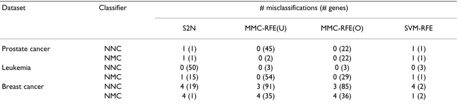
For each dataset, the minimum number of misclassifica-tions as well as the number of genes used are shown in Table 5. Both uncorrelated MMC-RFE and orthogonal MMC-RFE achieve zero misclassifications using a small number of genes for Prostate cancer and Leukemia, although S2N and SVM-RFE also perform comparably well. While S2N and MMC-RFE misclassify three or four test samples for Breast cancer, SVM-RFE yields fewer mis-classifications with NMC by using C = 0.001.
Tables 6, 7, 8 list the 10 top-ranked genes of orthogonal MMC-RFE and the corresponding ranks by S2N and SVM-RFE. Note that the lists of uncorrelated MMC-RFE are sim-ilar to those of orthogonal MMC-RFE, and hence omitted. For Prostate cancer, 7 genes are included in the list of 16 genes identified by Singh et al. [14] (Table 6). Of note,
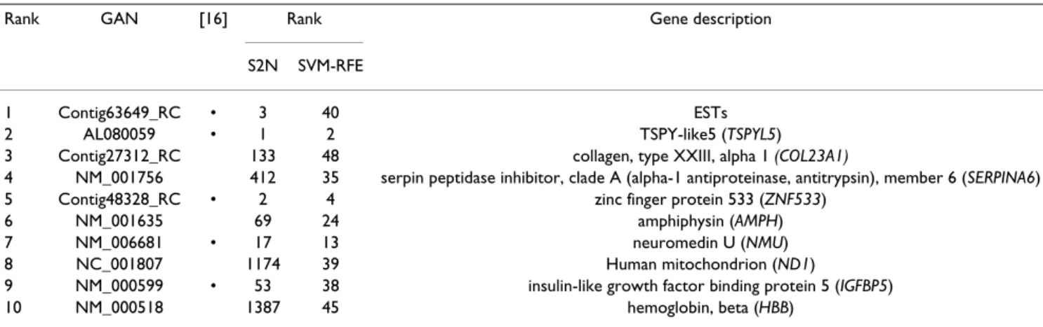
HPN (X07732) is ranked the first by all the three gene selection methods. It is known that hepsin, a cell surface serine protease, is overexpressed in prostate cancer and has been identified as a potential prostate-cancer biomar-ker [32,34-36]. HPN and CFD (M84526) are the two genes that are selected by uncorrelated MMC-RFE and achieve perfect classification with NMC. We can see that some of these genes are also highly ranked by S2N and SVM-RFE. Despite that there are differences in the pre-processing steps and gene selection criteria used, half the genes are included in the lists of the original studies for Leukemia and Breast cancer (Tables 7 and 8); the number of genes identified and used for prediction was 50 for Leukemia [3] and 70 for Breast cancer [16], respectively. It appears that the top-ranked genes of orthogonal MMC-RFE show a larger overlap with those of SVM-MMC-RFE than with those of S2N. Indeed, almost all the listed genes belong to the 50 top-ranked genes of SVM-RFE. On the other hand, some of them are assigned small ratio values Table 3: Performance comparison for multi-class datasets.
Classifier+Selection criterion Number of genes 10 20 30 50 100 MLL NMC+BW 11.5 ± 0.7 8.8 ± 0.6 7.4 ± 0.5 6.1 ± 0.5 5.6 ± 0.5 NMC+MMC-RFE(U) 7.0 ± 0.6 5.8 ± 0.5 5.1 ± 0.5 4.9 ± 0.5 4.0 ± 0.4 NMC+MMC-RFE(O) 6.4 ± 0.5 5.9 ± 0.5 5.6 ± 0.5 4.9 ± 0.4 4.4 ± 0.4 NMC+SVM-RFE(H) 26.9 ± 1.4 19.3 ± 1.2 15.5 ± 1.1 12.0 ± 0.8 9.1 ± 0.7 NMC+SVM-RFE(S) 28.0 ± 1.3 21.4 ± 1.1 16.6 ± 1.0 11.9 ± 0.8 7.9 ± 0.7 MMC+MMC-RFE(U) 6.8 ± 0.5 6.0 ± 0.5 5.2 ± 0.5 4.9 ± 0.5 4.0 ± 0.4 MMC+MMC-RFE(O) 6.4 ± 0.5 5.8 ± 0.5 5.6 ± 0.5 4.9 ± 0.4 4.5 ± 0.4 SVM+SVM-RFE(H) 31.3 ± 1.5 24.0 ± 1.4 18.3 ± 1.1 12.9 ± 0.8 7.9 ± 0.6 SVM+SVM-RFE(S) 26.2 ± 1.2 20.2 ± 1.1 14.4 ± 1.0 10.6 ± 0.8 6.8 ± 0.6 SRBCT NMC+BW 35.2 ± 1.4 22.1 ± 0.7 19.3 ± 0.7 10.5 ± 0.7 7.6 ± 0.6 NMC+MMC-RFE(U) 5.0 ± 0.5 3.0 ± 0.4 2.4 ± 0.3 2.2 ± 0.3 2.7 ± 0.3 NMC+MMC-RFE(O) 8.9 ± 0.7 6.0 ± 0.5 6.5 ± 0.5 6.8 ± 0.5 6.4 ± 0.5 NMC+SVM-RFE(H) 29.2 ± 1.2 22.9 ± 1.1 19.5 ± 1.0 15.7 ± 0.9 11.6 ± 0.7 NMC+SVM-RFE(S) 27.2 ± 1.2 21.9 ± 1.2 18.3 ± 1.0 14.2 ± 0.7 11.1 ± 0.8 MMC+MMC-RFE(U) 4.4 ± 0.5 2.5 ± 0.3 2.0 ± 0.3 1.7 ± 0.3 1.3 ± 0.2 MMC+MMC-RFE(O) 4.7 ± 0.5 4.1 ± 0.4 4.4 ± 0.4 3.5 ± 0.4 3.3 ± 0.4 SVM+SVM-RFE(H) 24.0 ± 1.3 14.2 ± 1.0 9.6 ± 0.7 6.3 ± 0.5 3.6 ± 0.4 SVM+SVM-RFE(S) 24.8 ± 1.4 12.7 ± 1.1 8.8 ± 0.8 5.1 ± 0.5 3.4 ± 0.4
The average error and standard error rates (%) for MLL and SRBCT, when the number of genes is {10, 20, 30, 50, 100}. SVM-RFE(S) shows the best result with respect to the C parameter; NMC+SVM-RFE(S): C = 0.1, SVM+SVM-RFE(S): C = 0.1 for MLL; NMC+SVM-RFE(S): C = 100, SVM+SVM-RFE(S): C = 1000 for SRBCT.
Page 10 of 18 by S2N. This may be due to the difference in gene
selec-tion approaches; MMC-RFE and SVM-RFE are multivari-ate, whereas S2N is univariate. It is interesting to note that the first rank gene of SVM-RFE for Breast cancer is PRAME (NM_006115), which in combination with TSPYL5 (AL080059) yields only one misclassification with NMC. The rank of PRAME by orthogonal MMC-RFE and S2N is 33 and 107, respectively. Overall, these results show that MMC-RFE can identify a small subset of discriminative genes that is quite consistent with previous studies.
Conclusion
In this paper, we have proposed a recursive gene selection method based on the MMC, and presented efficient and stable algorithms for MMC-RFE. The performance of MMC-RFE was extensively compared with that of SVM-RFE using nine cancer microarray datasets, including four multi-class datasets. We further compared the top-ranked genes selected by MMC-RFE with those of other gene selection methods, showing the validity of MMC-RFE.
The results suggest that MMC-RFE is less sensitive to noise and outliers due to the use of average margin, while the performance of SVM-RFE can be easily affected by them when applied to noisy, small sample size microarray data. Another advantage of MMC-RFE over SVM-RFE is that MMC-RFE naturally extends to multi-class cases. Further-more, MMC-RFE does not require the computation of the matrix inversion unlike LDA-RFE and MSE-RFE, and involves no parameters to be tuned.
This study has shown the effectiveness of the MMC for gene selection using microarray data. Our proposed algo-rithms can also be applied to proteomics and metabo-lomics datasets, and may be useful for biomarker discovery from such noisy data.
Methods
Maximum margin criterion
Linear discriminant analysis (LDA) aims to find a set of projection vectors which maximize the between-class scat-Table 4: Performance comparison for multi-class datasets (continued).
Classifier+Selection criterion Number of genes 10 20 30 50 100 CNS NMC+BW 31.1 ± 1.3 23.1 ± 1.2 20.1 ± 1.1 18.3 ± 1.0 15.9 ± 1.0 NMC+MMC-RFE(U) 27.2 ± 1.1 22.8 ± 0.9 21.9 ± 0.9 19.4 ± 0.8 16.8 ± 0.8 NMC+MMC-RFE(O) 24.4 ± 1.0 22.7 ± 0.8 22.1 ± 0.9 20.6 ± 0.9 18.9 ± 0.8 NMC+SVM-RFE(H) 45.6 ± 1.3 35.4 ± 1.0 33.3 ± 1.0 28.8 ± 0.9 24.9 ± 0.8 NMC+SVM-RFE(S) 45.4 ± 1.3 34.9 ± 1.0 32.5 ± 0.9 27.6 ± 0.8 24.6 ± 0.8 MMC+MMC-RFE(U) 27.6 ± 1.1 22.5 ± 0.9 21.3 ± 0.9 19.2 ± 0.8 16.9 ± 0.8 MMC+MMC-RFE(O) 24.4 ± 1.0 22.9 ± 0.8 22.2 ± 0.9 20.2 ± 0.9 19.4 ± 0.8 SVM+SVM-RFE(H) 54.0 ± 1.5 42.6 ± 1.4 36.8 ± 1.3 31.0 ± 0.9 25.2 ± 0.8 SVM+SVM-RFE(S) 47.3 ± 1.2 37.7 ± 1.1 32.6 ± 1.1 28.4 ± 1.0 26.6 ± 0.9 NCI60 NMC+BW 49.8 ± 1.2 44.0 ± 1.0 41.6 ± 1.0 39.1 ± 0.8 37.7 ± 0.7 NMC+MMC-RFE(U) 46.4 ± 0.8 38.9 ± 0.8 34.0 ± 0.9 29.8 ± 0.9 26.8 ± 0.7 NMC+MMC-RFE(O) 48.2 ± 0.9 39.6 ± 0.9 35.0 ± 0.9 31.6 ± 0.8 30.2 ± 0.9 NMC+SVM-RFE(H) 60.6 ± 1.0 51.4 ± 1.0 48.4 ± 1.0 43.4 ± 0.9 38.0 ± 0.8 NMC+SVM-RFE(S) 60.8 ± 1.0 52.2 ± 0.9 47.3 ± 1.0 41.3 ± 0.9 39.0 ± 0.9 MMC+MMC-RFE(U) 46.0 ± 0.9 37.3 ± 0.8 33.7 ± 0.8 29.0 ± 0.9 25.0 ± 0.7 MMC+MMC-RFE(O) 49.0 ± 1.0 38.6 ± 0.9 34.3 ± 0.9 30.4 ± 0.8 28.7 ± 0.9 SVM+SVM-RFE(H) 64.7 ± 1.2 54.3 ± 1.1 47.7 ± 1.0 42.0 ± 0.9 35.9 ± 0.9 SVM+SVM-RFE(S) 59.9 ± 1.1 50.3 ± 1.0 46.2 ± 1.0 42.8 ± 1.1 35.8 ± 0.9
The average error and standard error rates (%) for CNS and NCI60, when the number of genes is {10, 20, 30, 50, 100}. SVM-RFE(S) shows the best result with respect to the C parameter; NMC+SVM-RFE(S): C = 10, SVM+SVM-RFE(S): C = 0.1 for CNS; NMC+SVM-RFE(S): C = 100, SVM+SVM-RFE(S): C = 0.1 for NCI60.
Performance comparison for multi-class datasets Figure 3
Performance comparison for multi-class datasets. The average error rates (%) as a function of the number of genes from 1 to 100, for MLL and SRBCT.
0 20 40 60 80 100 0 5 10 15 20 25 30 35 40 45 50 Number of genes Error rate (%)
MLL
NMC+BW NMC+MMC−RFE(U) NMC+MMC−RFE(O) NMC+SVM−RFE(H) NMC+SVM−RFE(S) 0 20 40 60 80 100 0 5 10 15 20 25 30 35 40 45 50 Number of genes Error rate (%)SRBCT
NMC+BW NMC+MMC−RFE(U) NMC+MMC−RFE(O) NMC+SVM−RFE(H) NMC+SVM−RFE(S) 0 20 40 60 80 100 0 5 10 15 20 25 30 35 40 45 50 Number of genes Error rate (%)MLL
MMC+MMC−RFE(U) MMC+MMC−RFE(O) SVM+SVM−RFE(H) SVM+SVM−RFE(S) 0 20 40 60 80 100 0 5 10 15 20 25 30 35 40 45 50 Number of genes Error rate (%)SRBCT
MMC+MMC−RFE(U) MMC+MMC−RFE(O) SVM+SVM−RFE(H) SVM+SVM−RFE(S)Page 12 of 18 Performance comparison for multi-class datasets (continued)
Figure 4
Performance comparison for multi-class datasets (continued). The average error rates (%) as a function of the number of genes from 1 to 100, for CNS and NCI60.
0 20 40 60 80 100 0 10 20 30 40 50 60 70 80 Number of genes Error rate (%)
CNS
NMC+BW NMC+MMC−RFE(U) NMC+MMC−RFE(O) NMC+SVM−RFE(H) NMC+SVM−RFE(S) 0 20 40 60 80 100 0 10 20 30 40 50 60 70 80 Number of genes Error rate (%)NCI60
NMC+BW NMC+MMC−RFE(U) NMC+MMC−RFE(O) NMC+SVM−RFE(H) NMC+SVM−RFE(S) 0 20 40 60 80 100 0 10 20 30 40 50 60 70 80 Number of genes Error rate (%)CNS
MMC+MMC−RFE(U) MMC+MMC−RFE(O) SVM+SVM−RFE(H) SVM+SVM−RFE(S) 0 20 40 60 80 100 0 10 20 30 40 50 60 70 80 Number of genes Error rate (%)NCI60
MMC+MMC−RFE(U) MMC+MMC−RFE(O) SVM+SVM−RFE(H) SVM+SVM−RFE(S)Table 5: Performance comparison for independent test samples.
Dataset Classifier # misclassifications (# genes)
S2N MMC-RFE(U) MMC-RFE(O) SVM-RFE Prostate cancer NNC 1 (1) 0 (45) 0 (22) 1 (1) NMC 1 (1) 0 (2) 0 (22) 1 (1) Leukemia NNC 0 (50) 0 (3) 0 (3) 0 (3) NMC 1 (15) 0 (54) 0 (29) 1 (1) Breast cancer NNC 4 (19) 3 (91) 3 (85) 4 (2) NMC 4 (1) 4 (35) 4 (36) 1 (2) Minimum number of misclassifications and the number of genes used for Prostate cancer, Leukemia and Breast cancer. The C parameter of SVM-RFE was set to 0.01 for Prostate cancer, and to 0.001 for Leukemia and Breast cancer.
Table 6: Comparison of selected genes for Prostate cancer.
Rank GAN [14] Rank Gene description
S2N SVM-RFE
1 X07732 • 1 1 hepsin (transmembrane protease, serine 1) (HPN) 2 M30894 • 2 2 TCR gamma alternate reading frame protein (TARP) 3 M84526 • 3 89 complement factor D (adipsin) (CFD) 4 AL049969 • 4 65 PDZ and LIM domain 5 (PDLIM5) 5 X51345 38 5 jun B proto-oncogene (JUNB) 6 U21689 68 6 glutathione S-transferase pi (GSTP1) 7 M98539 • 297 15 prostaglandin D2 synthase 21kDa (brain) (PTGDS) 8 X17206 95 12 ribosomal protein S2 (RPS2)
9 D83018 • 6 41 NEL-like 2 (chicken) (NELL2)
10 AF065388 • 18 13 tetraspanin 1 (TSPAN1)
The 10 top-ranked genes of orthogonal MMC-RFE are listed in order of the rank; GAN: Gene Accession Number. Genes selected by Singh et al. [14] are denoted by •. C = 0.01 was used for SVM-RFE.
Table 7: Comparison of selected genes for Leukemia.
Rank GAN [3] Rank Gene description S2N SVM-RFE
1 M27891 • 1 2 cystatin C (CST3) 2 M28130 • 25 3 interleukin 8 (IL8)
3 M84526 • 5 1 D component of complement (adipsin) (DF) 4 M19507 131 7 myeloperoxidase (MPO) 5 Y00787 • 23 4 interleukin-8 precursor
6 M11722 71 41 deoxynucleotidyltransferase, terminal (DNTT)
7 X95735 • 2 11 zyxin (ZYX)
8 D88422 3 8 cystatin A (CSTA) 9 M27783 15 5 elastase 2, neutrophil (ELA2) 10 M96326 • 75 10 azurocidin 1 (AZU1)
The 10 top-ranked genes of orthogonal MMC-RFE are listed in order of the rank; GAN: Gene Accession Number. Genes selected by Golub et al. [3] are denoted by •. C = 0.001 was used for SVM-RFE.
Page 14 of 18 ter and simultaneously minimize the within-class scatter,
thereby achieving maximum discrimination [37]. The between-class scatter matrix Sb and the within-class
scatter matrix Sw are defined as
where c is the number of classes, mi and pi are the mean and a priori probability of class i, m is the total mean, and
Si is the covariance matrix of class i. Then, classical LDA
finds the projection vectors W by maximizing the Fisher criterion
J (W) = trace ((WT S
w W)-1 (WT Sb W)). (1)
By solving a generalized eigenvalue problem, the projec-tion vectors W can be found as the eigenvectors of Sb
corresponding to the largest eigenvalues. When the sam-ple size is smaller than the dimensionality of samsam-ples, however, Sw becomes singular and we cannot compute
Sb, which is a major drawback of classical LDA.
To overcome the singularity problem, several methods have been proposed e.g. in the field of computer vision, where the number of samples is usually much smaller than the dimensionality. A simple approach is to replace with the pseudo-inverse matrix . Another approach is to add some constant values to the diagonal
elements of Sw as Sw + μI, where μ > 0 and I is the identity matrix. However, each of these methods has its own draw-backs and does not scale well to high-dimensional data (see [11] for more details). Recently, Li et al. [11] pro-posed to use the maximum margin criterion (MMC) instead of (1) to find the projection vectors. The MMC is defined as
J (W) = trace (WT (S
b - Sw) W)). (2)
The projection vectors W = (w1,..., wd) which maximize (2) under the constraint that wk = 1, k = 1,..., d, can be
found as the eigenvectors of Sb - Sw corresponding to the largest eigenvalues. The advantage of using the MMC is that we need not compute the inverse of Sw, hence the sin-gularity problem can be easily avoided.
It is known that classical LDA can be related to SVM. Shashua [38] has shown that, in binary-class cases, the orientation and location of the hyperplane obtained by SVM is equivalent to the discriminant vector obtained by classical LDA using the samples on the margin. In other words, SVM can be viewed as sparsified LDA. Thus, noting that the MMC is different from classical LDA only in its constraint [11], the major difference between SVM and the MMC consists in that the hyperplane of SVM is con-structed only by the training samples closest to the deci-sion boundary, while the discriminant vector of the MMC is constructed so that the average margin computed by all training samples is maximized. They also lead to different problems to solve: a quadratic programming problem for the standard L2 SVM and an eigenvalue problem for the MMC. Note that for L1 SVM, it can be reduced to a linear programming problem (see [9] and references therein).
S m m m m S S b i i i T i c w i i i c p p = − − = = =
∑
∑
( )( ) , , 1 1 Sw−1 Sw−1 Sw−1 Sw+ wkTTable 8: Comparison of selected genes for Breast cancer.
Rank GAN [16] Rank Gene description
S2N SVM-RFE
1 Contig63649_RC • 3 40 ESTs 2 AL080059 • 1 2 TSPY-like5 (TSPYL5) 3 Contig27312_RC 133 48 collagen, type XXIII, alpha 1 (COL23A1)
4 NM_001756 412 35 serpin peptidase inhibitor, clade A (alpha-1 antiproteinase, antitrypsin), member 6 (SERPINA6) 5 Contig48328_RC • 2 4 zinc finger protein 533 (ZNF533)
6 NM_001635 69 24 amphiphysin (AMPH) 7 NM_006681 • 17 13 neuromedin U (NMU) 8 NC_001807 1174 39 Human mitochondrion (ND1)
9 NM_000599 • 53 38 insulin-like growth factor binding protein 5 (IGFBP5) 10 NM_000518 1387 45 hemoglobin, beta (HBB)
The 10 top-ranked genes of orthogonal MMC-RFE are listed in order of the rank; GAN: Gene Accession Number. Genes selected by van't Veer et al. [16] are denoted by •. C = 0.001 was used for SVM-RFE.
MMC-RFE algorithms for gene selection
The idea of recursive feature elimination (RFE) [6] is to recursively remove genes using the absolute weights of the discriminant vector or hyperplane, which reflect the sig-nificance of the genes for classification. The process starts by training the classifier using all genes. Then, the genes are ranked according to the absolute weights, and those genes with the smallest absolute weights are removed. The classifier is retrained with the remaining genes. This proc-ess is repeated until the maximum classification accuracy is obtained or the number of genes reaches a predeter-mined value. The RFE approach has recently been shown to be effective not only with SVM but also with penalized logistic regression [39] and ridge regression [10].
Here, we propose a recursive gene selection method based on the MMC. The MMC is computationally more efficient and stable than classical LDA, yet it does not scale well to high-dimensional data. When we consider using RFE with the MMC, it is computationally intensive to perform the eigenvalue decomposition (EVD) of the matrix of the gene size in a recursive manner. To overcome the problem of high dimensionality, we first remove the null space of the total scatter matrix via singular value decomposition (SVD) [40], thereby reduce the dimensionality of the data to n - 1, where n is the number of samples, and then max-imize the MMC in the reduced space. Let X denote the gene expression matrix of size p × n, where p is the number of genes. Then, the total scatter matrix St can be expressed as
where
and e = (1,1,..., 1)T is an n-dimensional vector. Let us
assume that p > n and perform the reduced SVD of as
where = diag (λ1,..., λn) with decreasing non-negative values, and and are p × n and n × n orthonormal matrices. Since the rank of St is n - 1, i.e. λn = 0, we can rewrite (3) as
= UΛVT,
where Λ= diag (λ1,..., λn - 1), and U and V are p × (n - 1) and n × (n - 1) matrices consisting of the corresponding (n
- 1) vectors. Thus, we can reduce the dimension by pro-jecting X onto the (n - l)-dimensional space as
Z = Λ-1 UT X. (4)
Then, we may maximize the MMC on Z, which is a (n - 1) × n matrix. Here, we require W to be orthogonal, i.e. WT
W = I, in the reduced space. Once the discriminant vectors
W of size (n - 1) × d is obtained, they are projected back onto the original p-dimensional space by
= U Λ-1 W, (5)
where is of size p × d. Finally, gene selection can be performed using . When using (4), we can show that the number of the discriminant vectors that correspond to the positive eigenvalues is at most c - 1. Because the eigen-values reflect the discrimination ability, we use the (c - 1) discriminant vectors corresponding to the positive eigen-values, i.e. d is set to c - 1, and discard those corresponding to the negative eigenvalues.
Li et al. [11] proposed another efficient method to com-pute the projection vectors of the MMC. It is interesting to note that the MMC is related to uncorrelated LDA (ULDA), and we can find that the Li's method is the same as the ULDA algorithm proposed by Ye [41]. It can be shown that in (5) maximizes the MMC on X under the constraint that T S
t = I, and our method turns out to
be equivalent to the ULDA algorithm. Hence, we call the algorithm based on (4) uncorrelated MMC-RFE.
This study also explores the following projection instead of (4):
Z = UT X. (6)
After obtaining the discriminant vectors W by maximizing the MMC on Z, they are projected back onto the original p-dimensional space by
= U W. (7)
Note that no discriminant information is lost in the case of (6) [42]. It can be shown that in (7) maximizes the MMC on X under the constraint that T = I. We call
the algorithm based on (6) orthogonal MMC-RFE. We see that the difference between (4) and (6) results in the dif-ferent constraints of the MMC on X.
St = XXT, X= 1 X−me n T ( ), X X =U VΛΛ T (3), ΛΛ U V X W W W W W W W W W W
Page 16 of 18 The uncorrelated MMC-RFE and orthogonal MMC-RFE
algorithms are summarized in Figures 5 and 6, respec-tively. They are different in step 3 and step 6. The main computation of both algorithms consists of the SVD of a p × n matrix at step 2 and the EVD of a (n - 1) × (n - 1) matrix at step 5. Thus, the algorithms are feasible in the case of high dimensionality and small sample size, i.e. large p and small n. As is shown, the MMC-RFE algorithms can naturally treat multi-class cases, in which the weight of gene j can be defined as the sum of the absolute weights of c - 1 discriminant vectors in , i.e. . The maximum of the absolute weights, i.e. maxk = 1,..., c - 1 | jk|, may also be useful. Note that the uncorrelated MMC-RFE algorithm switches to orthogonal MMC-RFE at q = n - 1, where q is the number of remaining genes during elimina-tion. Hence, our algorithm and the ULDA algorithm may select different genes when q ≤ n - 1.
MMC classifier
The MMC classifier performs nearest mean classification in the projected space, i.e. the class label y of a test sample
x is predicted as
where mi is the mean of class i. Since we perform classifi-cation using at most 100 genes in the experiments, the dis-criminant vectors W were computed by directly maximizing the MMC under the orthogonality constraint.
S2N ratio and BW ratio
For each gene j, the S2N ratio [4] is defined as
where , and , denote the means and
standard deviations of two classes, respectively. Top-ranked genes are those with the largest values of S2N(j). The BW ratio [5] can be defined as
where and respectively denote the average expression level of gene j for class k and the overall average expression level of gene j across all samples, yi denotes the class of sample i, and I (·) is the indicator function. W
∑
kc−=11|wjk| w ˆ arg min || ( ) || , y i T i = W x−m 2 S N2 1 2 1 2 ( ) | |, ( ) ( ) ( ) ( ) j j j j j = − + μ μ σ σ μj ( )1 μj ( )2 σj ( )1 σj ( )2 BW( ) ( )( . . ) ( )( . ) , ( ) ( ) j I y k x x I y k x x i j k j k i i ij j k k i = = − = −∑
∑
∑
∑
2 2 x.( )jk x.jThe uncorrelated MMC-RFE algorithm Figure 5
ranked genes with the largest values of BW(j) are used for classification.
Authors' contributions
SN designed the experiments, carried out all the analysis, and drafted the manuscript. SK supervised the project. All authors read and approved the final manuscript.
Acknowledgements
This work was supported by KAKENHI (Grant-in-Aid for Scientific Research) on Priority Areas "Comparative Genomics" from the Ministry of Education, Culture, Sports, Science and Technology of Japan.
References
1. Stolovitzky G: Gene selection in microarray data: the elephant,
the blind men and our algorithms. Curr Opin Struct Biol 2003,
13:370-376.
2. Cuperlovic-Culf M, Belacel N, Ouellette RJ: Determination of tumour
marker genes from gene expression data. Drug Discov Today 2005,
10:429-437.
3. Golub TR, Slonim DK, Tamayo P, Huard C, Gaasenbeek M, Mesirov JP, Coller H, Loh ML, Downing JR, Caligiuri MA, Bloomfield CD, Lander ES: Molecular classification of cancer: class discovery and class
pre-diction by gene expression monitoring. Science 1999, 286:531-537.
4. Furey TS, Cristianini N, Duffy N, Bednarski DW, Schummer M, Haussler D: Support vector machine classification and validation of cancer
tissue samples using microarray expression data. Bioinformatics
2000, 16:906-914.
5. Dudoit S, Fridlyand J, Speed TP: Comparison of discrimination
meth-ods for the classification of tumors using gene expression data. J
Amer Statist Assoc 2002, 97:77-87.
6. Guyon I, Weston J, Barnhill S, Vapnik V: Gene selection for cancer
classification using support vector machines. Mach Learn 2002,
46:389-422.
7. Rakotomamonjy A: Variable selection using SVM-based criteria. J Mach Learn Res 2003, 3:1357-1370 [http://jmlr.csail.mit.edu/papers/v3/ rakotomamonjy03a.html].
8. Weston J, Elisseeff A, Schölkopf B, Tipping M: Use of the zero-norm
with linear models and kernel methods. J Mach Learn Res 2003,
3:1439-1461 [http://jmlr.csail.mit.edu/papers/v3/weston03a.html]. 9. Zhang HH, Ahn J, Lin X, Park C: Gene selection using support vector
machines with non-convex penalty. Bioinformatics 2006, 22:88-95.
10. Li F, Yang Y: Analysis of recursive gene selection approaches from
microarray data. Bioinformatics 2005, 21:3741-3747.
11. Li H, Jiang T, Zhang K: Efficient and robust feature extraction by
maximum margin criterion. IEEE Trans Neural Netw 2006,
17:157-165.
12. Ambroise C, McLachlan GJ: Selection bias in gene extraction on the
basis of microarray gene-expression data. Proc Natl Acad Sci USA
2002, 99:6562-6566.
13. Alon U, Barkai N, Notterman DA, Gish K, Ybarra S, Mack D, Levine AJ: Broad patterns of gene expression revealed by clustering analy-sis of tumor and normal colon tissues probed by oligonucleotide
arrays. Proc Natl Acad Sci USA 1999, 96:6745-6750.
14. Singh D, Febbo PG, Ross K, Jackson DG, Manola J, Ladd C, Tamayo P, Ren-shaw AA, D'Amico AV, Richie JP, Lander ES, Loda M, Kantoff PW, Golub TR, Sellers WR: Gene expression correlates of clinical prostate
cancer behavior. Cancer Cell 2002, 1:203-209.
15. Pomeroy SL, Tamayo P, Gaasenbeek M, Sturla LM, Angelo M, McLaughlin ME, Kim JYH, Goumnerova LC, Black PM, Lau C, Allen JC, Zagzag D, Olson JM, Curran T, Wetmore C, Biegel JA, Poggio T, Mukherjee S, Rifkin R, Califano A, Stolovitzky G, Louis DN, Mesirov JP, Lander ES, Golub TR: Prediction of central nervous system embryonal tumour
out-come based on gene expression. Nature 2002, 415:436-442.
16. van't Veer LJ, Dai H, van de Vijver MJ, He YD, Hart AAM, Mao M, Peterse HL, van der Kooy K, Marton MJ, Witteveen AT, Schreiber GJ, Kerkhoven RM, Roberts C, Linsley PS, Bernards R, Friend SH: Gene expression
profiling predicts clinical outcome of breast cancer. Nature 2002,
415:530-536.
17. Armstrong SA, Staunton JE, Silverman LB, Pieters R, den Boer ML, Minden MD, Sallan SE, Lander ES, Golub TR, Korsmeyer SJ: MLL translocations specify a distinct gene expression profile that distinguishes a
unique leukemia. Nat Genet 2002, 30:41-47.
18. Khan J, Wei JS, Ringnér M, Saal LH, Ladanyi M, Westermann F, Berthold F, Schwab M, Antonescu CR, Peterson C, Meltzer PS: Classification and diagnostic prediction of cancers using gene expression profiling
and artificial neural networks. Nat Med 2001, 7:673-679.
19. Ross DT, Scherf U, Eisen MB, Perou CM, Rees C, Spellman P, Iyer V, Jef-frey SS, Van de Rijn M, Waltham M, Pergamenschikov A, Lee JCF, Lashkari D, Shalon D, Myers TG, Weinstein JN, Botstein D, Brown PO: System-atic variation in gene expression patterns in human cancer cell
lines. Nat Genet 2000, 24:227-235.
The orthogonal MMC-RFE algorithm Figure 6
Publish with BioMed Central and every scientist can read your work free of charge
"BioMed Central will be the most significant development for disseminating the results of biomedical researc h in our lifetime."
Sir Paul Nurse, Cancer Research UK Your research papers will be:
available free of charge to the entire biomedical community peer reviewed and published immediately upon acceptance cited in PubMed and archived on PubMed Central yours — you keep the copyright
Submit your manuscript here:
http://www.biomedcentral.com/info/publishing_adv.asp
BioMedcentral
Page 18 of 18
20. Colon cancer dataset [http://microarray.princeton.edu/oncology/affy
data/index.html]
21. Cancer Program Data Sets [http://www.broad.mit.edu/cgi-bin/can
cer/datasets.cgi]
22. Rosetta Inpharmatics [http://www.rii.com/publications/2002/
vantveer.html]
23. Microarray Project [http://research.nhgri.nih.gov/microarray/Supple
ment/]
24. Stanford NCI60 Cancer Microarray Project
[http://genome-www.stanford.edu/nci60/]
25. Ramaswamy S, Tamayo P, Rifkin R, Mukherjee S, Yeang CH, Angelo M, Ladd C, Reich M, Latulippe E, Mesirov JP, Poggio T, Gerald W, Loda M, Lander ES, Golub TR: Multiclass cancer diagnosis using tumor gene
expression signatures. Proc Natl Acad Sci USA 2001, 98:15149-15154.
26. The Spider Library for MATLAB [http://www.kyb.tuebingen.mpg.de/
bs/people/spider/]
27. Wessels LFA, Reinders MJT, Hart AAM, Veenman CJ, Dai H, He YD, van't Veer LJ: A protocol for building and evaluating predictors of
dis-ease state based on microarray data. Bioinformatics 2005,
21:3755-3762.
28. Huang TM, Kecman V: Gene extraction for cancer diagnosis by
sup-port vector machines – An improvement. Artif Intell Med 2005,
35:185-194.
29. Duda RO, Hart PE, Stork DG: Pattern Classification 2nd edition. New York: Wiley; 2001.
30. Xu J, Zhang X, Li Y: Kernel MSE algorithm: A unified framework for
KFD, LS-SVM and KRR. In Proceedings of the International Joint
Confer-ence on Neural Networks: 15–19 July 2001 Washington, DC, IEEE; 2001:1486-1491.
31. Michiels S, Koscielny S, Hill C: Prediction of cancer outcome with
microarrays: a multiple random validation strategy. Lancet 2005,
365:488-492.
32. Welsh JB, Sapinoso LM, Su AI, Kern SG, Wang-Rodriguez J, Moskaluk CA, Frierson HF Jr, Hampton GM: Analysis of gene expression identifies candidate markers and pharmacological targets in prostate
can-cer. Cancer Res 2001, 61:5974-5978.
33. Prostate cancer data from GNF [http://www.gnf.org/cancer/pros
tate]
34. Dhanasekaran SM, Barrette TR, Ghosh D, Shah R, Varambally S, Kurachi K, Pienta KJ, Rubin MA, Chinnaiyan AM: Delineation of prognostic
biomarkers in prostate cancer. Nature 2001, 412:822-826.
35. Luo J, Duggan DJ, Chen Y, Sauvageot J, Ewing CM, Bittner ML, Trent JM, Isaacs WB: Human prostate cancer and benign prostatic
hyperpla-sia: Molecular dissection by gene expression profiling. Cancer Res
2001, 61:4683-4688.
36. Magee JA, Araki T, Patil S, Ehrig T, True L, Humphrey PA, Catalona WJ, Watson MA, Milbrandt J: Expression profiling reveals hepsin
overex-pression in prostate cancer. Cancer Res 2001, 61:5692-5696.
37. Fukunaga K: Introduction to Statistical Pattern Recognition 2nd edition. Bos-ton, MA: Academic Press; 1990.
38. Shashua A: On the relationship between the support vector machine for classification and sparsified Fisher's linear
discrimi-nant. Neural Processing Lett 1999, 9:129-139.
39. Zhu J, Hastie T: Classification of gene microarrays by penalized
logistic regression. Biostatistics 2004, 5:427-443.
40. Golub GH, Van Loan CF: Matrix Computations 3rd edition. Baltimore, MD: Johns Hopkins University Press; 1996.
41. Ye J: Characterization of a family of algorithms for generalized
discriminant analysis on undersampled problems. J Mach Learn Res
2005, 6:483-502 [http://jmlr.csail.mit.edu/papers/v6/ye05a.html]. 42. Yang J, Yang JY: Why can LDA be performed in PCA transformed
space? Pattern Recognition 2003, 36:563-566 [http://dx.doi.org/10.1016/