Compounding a class of Rayleigh
distributions: an objective Bayesian approach
by
Renier van Rooyen
December 2015
Thesis presented in fulfilment of the requirements for the degree of Master of Science in the Faculty of Science at Stellenbosch University
Declaration
By submitting this thesis/dissertation electronically, I declare that the entirety of the work contained therein is my own, original work, that I am the sole author thereof (save to the extent explicitly otherwise stated), that reproduction and publication thereof by Stellenbosch
University will not infringe any third party rights and that I have not previously in its entirety or in part submitted it for obtaining any qualification.
December 2015
Copyright © 2015 Stellenbosch University
“To those who do not know mathematics it is difficult to get across a real feeling as to the beauty, the deepest beauty, of nature. If you want to learn about nature, to appreciate nature, it is necessary to understand the language that she speaks in.”
UNIVERSITY OF STELLENBOSCH
Abstract
Compounding a class of Rayleigh distributions: an objective Bayesian approach
by Renier van Rooyen
In this work, Bayesian estimation in the context of parametric survival analysis is con-sidered. A class of models derived by compounding and generalising the Rayleigh dis-tribution is regarded. These models are well suited to survival analysis settings where the hazard rate is characterised by a sharp increase over time. An objective Bayesian approach is followed, whereby non-informative prior distribution selection leads to the use of the Jeffreys, the reference and the probability matching priors. Bayesian point estimators are derived using two symmetric loss functions, namely absolute error and squared error, as well as two asymmetric loss functions, namely linear exponential and general entropy. The resulting models and estimators are showcased in a simulation study by generating right censored lifetime data from the various compound models and utilising the Metropolis-Hastings algorithm to draw realisations from the corresponding posterior distributions, since closed-form expressions for these cannot be found. Obtain-ing the Fisher information plays a crucial part in derivObtain-ing the non-informative priors. In cases where it cannot be analytically evaluated, an adaptive quadrature routine is used for the numerical approximation of some of the elements in the Fisher information. An application to data sets from practice concludes the exposition of the compound Rayleigh models of interest.
UNIVERSITEIT VAN STELLENBOSCH
Opsomming
Compounding a class of Rayleigh distributions: an objective Bayesian approach
deur Reniervan Rooyen
In hierdie tesis, word Bayes-beraming beskou in die konteks van parametriese oorle-wingsanalise. ’n Klas modelle wat afgelei is deur samestelling en veralgemening van die Rayleigh-verdeling, word beskou. Hierdie modelle is toepaslik in oorlewingsanalise-scenarios waar die gevaarfunksie beskryf word deur ’n skerp toename oor tyd. ’n Ob-jektiewe Bayes-benadering word gevolg en die toepaslike keuse van nie-inligtinggewende prior-verdelings lei na die gebruik van die Jeffreys-, die verwysings- en die waarskyn-likheidspassende priors. Bayes puntberamers word afgelei met inagneming van twee simmetriese verliesfunksies, naamlik absolute fout en kwadratiese fout, sowel as twee asimmetriese verliesfunksies, naamlik lineˆer eksponensieel en algemene entropie. Die gevolglike modelle en beramers word ten toon gestel in ’n simulasiestudie deur regs-gesensoreerde leeftyd-data te genereer vanuit die verskeie saamgestelde modelle en dan die Metropolis-Hastings algoritme te gebruik om realiserings vanuit die ooreenstem-mende posterior-verdelings te verkry, aangesien oplossings vir hierdie funksies nie in geslote vorm gevind kan word nie. Die bepaling van die Fisher-inligting speel ‘n kar-dinale rol in die afleiding van die nie-inligtinggewende priors. In gevalle waar dit nie analities evalueer kan word nie, word ’n aanpassende kwadratuurroetine gebruik vir die numeriese benaderings van sommige elemente in die Fisher-inligting. Laastens word die uiteensetting van die saamgestelde Rayleigh modelle afgesluit deur die toepassing op twee datastelle uit die praktyk.
Acknowledgements
I would like to express my sincerest gratitude to the DST-NRF Centre of Excellence in Epidemiological Modelling and Analysis (SACEMA) and the Institute of Applied Statistics (IAS) for providing guidance and financial support, and accordingly making my M.Sc. studies possible. (Opinions expressed and conclusions arrived at, are those of the author and are not necessarily to be attributed to SACEMA or the IAS.)
I want to thank Professor Paul Mostert unreservedly for the expertise, continuous help, motivation, encouragement and enormous amounts of patience. I also want to thank Dr. Martin Nieuwoudt as well as others at SACEMA for many ideas and enthusiasm. Lastly my friends and loved ones, especially my parents, Club 84 and Ilani, for inspiring me to never give up.
Contents
Declaration of Authorship i Abstract iii Opsomming iv Acknowledgements v Contents vi List of Figures ixList of Tables xii
Abbreviations xiv
Symbols xv
1 Introduction 1
2 Survival analysis and the Bayesian method 4
2.1 Concepts in survival analysis . . . 4
2.1.1 Important parameters in a survival analysis . . . 5
2.1.2 Different approaches to parameter estimation . . . 7
2.2 Overview of the Bayesian method . . . 9
2.2.1 Updating prior information to the posterior distribution . . . 10
2.2.2 Loss functions and Bayesian estimators . . . 13
2.2.2.1 Risk and estimation in the Bayesian setting . . . 13
2.2.2.2 Quantifying loss in estimation . . . 14
2.2.2.3 Derivations of Bayesian estimators . . . 18
2.2.3 The Fisher information . . . 19
2.2.3.1 Background and relevance to current work . . . 19
2.2.3.2 Numerical approximation of the Fisher information . . . 20
2.2.4 Non-informative approach to prior distribution specification . . . . 22
2.2.4.1 The Jeffreys prior . . . 23
Contents
2.2.4.3 The probability matching prior . . . 26
2.2.5 Simulating the posterior distribution . . . 27
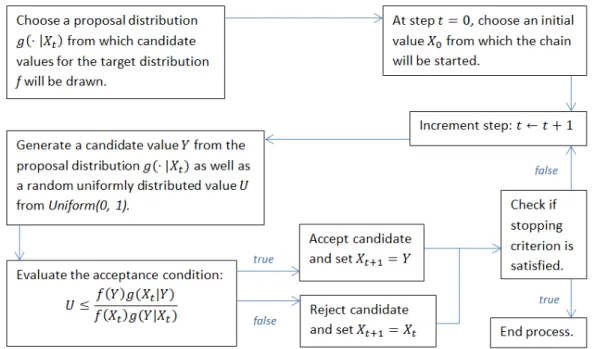
2.2.5.1 MCMC and the Metropolis-Hastings algorithm . . . 28
2.2.5.2 Monitoring convergence of Markov chains . . . 30
2.3 Philosophical considerations . . . 33
2.4 Summary . . . 35
3 The Rayleigh distribution and its compounded forms 37 3.1 The Rayleigh as a lifetime distribution . . . 37
3.2 Compounding and generalising the Rayleigh distribution . . . 40
3.2.1 Background of Rayleigh modifications . . . 40
3.2.1.1 Compound distributions . . . 41
3.2.1.2 Generalised distributions . . . 42
3.2.2 Compounding and generalising the Rayleigh model . . . 44
3.2.2.1 Compounding with respect to the exponential distribution 45 3.2.2.2 Compounding with respect to the Gamma distribution . 46 3.2.2.3 Generalising the compounded distributions . . . 47
3.2.3 Expansion and estimation of the compounded Rayleigh models . . 49
3.3 Simulation studies on the compounded Rayleigh mo-dels . . . 49
3.3.1 Simulating random samples from Rayleigh models . . . 50
3.3.2 Simulation study methods and quantities of interest . . . 50
3.4 Summary . . . 53
4 Simulation study of compound models 55 4.1 The CRE model . . . 55
4.1.1 Model characteristics . . . 55
4.1.2 Prior and posterior distributions . . . 57
4.1.3 Bayesian estimators of the parameter . . . 58
4.1.4 Simulation results . . . 59
4.1.5 Discussion . . . 70
4.2 The CRG model . . . 71
4.2.1 Model characteristics . . . 71
4.2.2 Prior and posterior distributions . . . 73
4.2.2.1 Derivation of the Jeffreys prior . . . 73
4.2.2.2 Derivation of the reference priors . . . 74
4.2.2.3 Derivation of the probability matching prior . . . 77
4.2.2.4 Derivation of posterior distributions . . . 78
4.2.3 Bayesian estimators of the parameters . . . 79
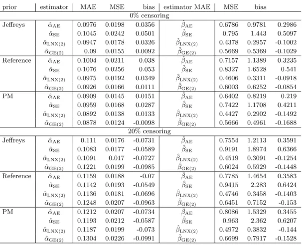
4.2.4 Simulation results . . . 80
4.2.5 Discussion . . . 97
4.3 Summary . . . 98
5 Simulation study of compounded and generalised models 100 5.1 The GCRE model . . . 100
5.1.1 Model characteristics . . . 100
5.1.2 Prior and posterior distributions . . . 103
Contents
5.1.4 Simulation results . . . 105
5.1.5 Discussion . . . 125
5.2 The GCRG model . . . 126
5.2.1 Model characteristics . . . 126
5.2.2 Prior and posterior distributions . . . 129
5.2.3 Bayesian estimators of the parameters . . . 131
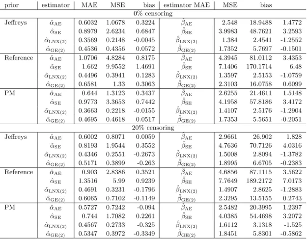
5.2.4 Simulation results . . . 132
5.2.5 Discussion . . . 163
5.3 Summary . . . 164
6 Illustration and application of the results 166 6.1 Motivation and methods . . . 166
6.2 Model comparisons using the DIC . . . 167
6.3 Wind speed data . . . 169
6.4 Gastrointestinal cancer data . . . 180
7 Conclusions 186 7.1 The effect of censoring on estimators . . . 186
7.2 Comparison of loss functions . . . 187
7.3 Comparison of prior distributions . . . 188
7.4 Comparison of compound Rayleigh models . . . 188
7.5 Shortcomings and further work . . . 189
7.5.1 Shortcomings . . . 189
7.5.2 Potential for future work . . . 190
A Additional definitions 191 A.1 The inverse transform method . . . 191
A.2 The Beta prime distribution . . . 191
B Software code 193 B.1 R code for distributions, priors and posteriors . . . 193
B.2 R code for Metropolis-Hastings algorithms . . . 197
B.3 R code for simulation studies . . . 203
B.4 R code for plots . . . 218
List of Figures
2.1 Visual depiction of loss functions . . . 17
2.2 Metropolis-Hastings algorithm flowchart . . . 29
3.1 Rayleigh density for various values of θ. . . 38
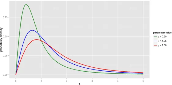
3.2 CRE density for various values of γ . . . 45
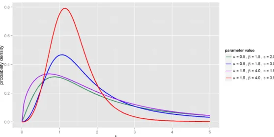
3.3 CRG density for various values of α and β . . . 46
3.4 GCRE density for various values ofγ and c . . . 48
3.5 GCRG density for various values of α,β and c . . . 48
4.1 Hazard rate of CRE model . . . 56
4.2 Bayesian estimates of CRE (γ = 0.5) . . . 61
4.3 Hazard rate estimates of CRE (γ = 0.5) . . . 62
4.4 Bayesian estimates of CRE (γ = 1.25) . . . 64
4.5 Hazard rate estimates of CRE (γ = 1.25) . . . 65
4.6 Bayesian estimates of CRE (γ = 1.25 and n= 30) . . . 66
4.7 Hazard rate estimates of CRE (γ = 1.25 and n= 30) . . . 67
4.8 Bayesian estimates of CRE (γ = 2) . . . 68
4.9 Hazard rate estimates of CRE (γ = 2) . . . 69
4.10 Hazard rate of CRG model . . . 73
4.11 Bayesian estimates of CRG (α= 0.5 and β = 1.5) . . . 81
4.12 MSE vs bias of CRG (α= 0.5 andβ = 1.5) . . . 82
4.13 Hazard rate estimates of CRG (α = 0.5 andβ = 1.5) . . . 83
4.14 Bayesian estimates of CRG (α= 1.5 and β = 4) . . . 85
4.15 MSE vs bias of CRG (α= 1.5 andβ = 4) . . . 86
4.16 Hazard rate estimates of CRG (α = 1.5 andβ = 4) . . . 87
4.17 Bayesian estimates of CRG (α= 0.5 and β = 3.5) . . . 89
4.18 MSE vs bias of CRG (α= 0.5 andβ = 3.5) . . . 90
4.19 Hazard rate estimates of CRG (α = 0.5 andβ = 3.5) . . . 91
4.20 Bayesian estimates of CRG (α= 0.5, β= 3.5 and n= 30) . . . 93
4.21 MSE vs bias of CRG (α= 0.5,β = 3.5 andn= 30) . . . 94
4.22 Hazard rate estimates of CRG (α = 0.5,β= 3.5 and n= 30) . . . 95
5.1 Hazard rate of GCRE model . . . 101
5.2 Bayesian estimates of GCRE (γ = 0.5 andc= 3) . . . 107
5.3 MSE vs bias of GCRE (γ = 0.5 and c= 3) . . . 108
5.4 Hazard rateestimates of GCRE (γ= 0.5 and c= 3) . . . 109
5.5 Bayesian estimates of GCRE (γ = 1 and c= 4) . . . 110
List of Figures
5.7 Hazard rate estimates of GCRE (γ = 1 and c= 4) . . . 112
5.8 Bayesian estimates of GCRE (γ = 1,c= 4 and n= 30) . . . 113
5.9 MSE vs bias of GCRE (γ = 1, c= 4 and n= 30) . . . 114
5.10 Hazard rate estimates of GCRE (γ = 1,c= 4 and n= 30) . . . 115
5.11 Bayesian estimates of GCRE (γ = 0.5 andc= 4) . . . 116
5.12 MSE vs bias of GCRE (γ = 0.5 and c= 4) . . . 117
5.13 Hazard rate estimates of GCRE (γ = 0.5 andc= 4) . . . 118
5.14 Bayesian estimates of GCRE (γ = 1 and c= 3) . . . 119
5.15 MSE vs bias of GCRE (γ = 1 and c= 3) . . . 120
5.16 Hazard rate estimates of GCRE (γ = 1 and c= 3) . . . 121
5.17 Bayesian estimates of GCRE (γ = 0.5 andc= 5) . . . 122
5.18 MSE vs bias of GCRE (γ = 0.5 and c= 5) . . . 123
5.19 Hazard rate estimates of GCRE (γ = 0.5 andc= 5) . . . 124
5.20 Hazard rate of GCRG model . . . 126
5.21 Bayesian estimates of GCRG (α= 0.5,β = 1.5 and c= 2) . . . 133
5.22 MSE vs bias plots,α parameter, GCRG (α = 0.5 andβ = 1.5 andc= 2) 134 5.23 MSE vs bias plots,β parameter, GCRG (α= 0.5 and β= 1.5 and c= 2) . 135 5.24 MSE vs bias plots,cparameter, GCRG (α= 0.5 and β= 1.5 and c= 2) . 136 5.25 Hazard rate estimates of GCRG (α= 0.5, β= 1.5 and c= 2) . . . 137
5.26 Bayesian estimates of GCRG (α= 0.5,β = 1.5 and c= 3) . . . 139
5.27 MSE vs bias plots,α parameter, GCRG (α = 0.5 andβ = 1.5 andc= 3) 140 5.28 MSE vs bias plots,β parameter, GCRG (α= 0.5 and β= 1.5 and c= 3) . 141 5.29 MSE vs bias plots,cparameter, GCRG (α= 0.5 and β= 1.5 and c= 3) . 142 5.30 Hazard rate estimates of GCRG (α= 0.5, β= 1.5 and c= 3) . . . 143
5.31 Bayesian estimates of GCRG (α= 0.5,β = 1.5,c= 3 and n= 30) . . . . 145
5.32 MSE vs bias plots, α parameter, GCRG (α = 0.5, β = 1.5, c = 3 and n= 30) . . . 146
5.33 MSE vs bias plots, β parameter, GCRG (α = 0.5, β = 1.5, c = 3 and n= 30) . . . 147
5.34 MSE vs bias plots, c parameter, GCRG (α = 0.5, β = 1.5, c = 3 and n= 30) . . . 148
5.35 Hazard rate estimates of GCRG (α= 0.5, β= 1.5,c= 3 and n= 30) . . . 149
5.36 Bayesian estimates of GCRG (α= 1.5,β = 4 and c= 1.5) . . . 151
5.37 MSE vs bias plots,α parameter, GCRG (α = 1.5 andβ = 4 andc= 1.5) 152 5.38 MSE vs bias plots,β parameter, GCRG (α= 1.5 and β= 4 and c= 1.5) . 153 5.39 MSE vs bias plots,cparameter, GCRG (α= 1.5 and β= 4 and c= 1.5) . 154 5.40 Hazard rate estimates of GCRG (α= 1.5, β= 4 and c= 1.5) . . . 155
5.41 Bayesian estimates of GCRG (α= 1.5,β = 4 and c= 3.5) . . . 157
5.42 MSE vs bias plots,α parameter, GCRG (α = 1.5 andβ = 4 andc= 3.5) 158 5.43 MSE vs bias plots,β parameter, GCRG (α= 1.5 and β= 4 and c= 3.5) . 159 5.44 MSE vs bias plots,cparameter, GCRG (α= 1.5 and β= 4 and c= 1.5) . 160 5.45 Hazard rate estimates of GCRG (α= 1.5, β= 4 and c= 3.5) . . . 161
6.1 Hazard rate estimates for wind data using CRE and GCRE models . . . . 177
6.2 Hazard rate estimates for wind data using CRG model . . . 178
6.3 Hazard rate estimates for wind data using GCRG model . . . 179
List of Figures
List of Tables
2.1 General form of Bayesian estimators under loss functions . . . 18
3.1 Inverse transform method results . . . 50
4.1 MAE, MSE and bias for CRE, γ = 0.5 . . . 62
4.2 MAE, MSE and bias for CRE, γ = 1.25 . . . 65
4.3 MAE, MSE and bias for CRE, γ = 1.25 andn= 30 . . . 67
4.4 MAE, MSE and bias for CRE, γ = 2 . . . 69
4.5 MAE, MSE and bias for CRG, (α, β) = (0.5,1.5) . . . 84
4.6 MAE, MSE and bias for CRG, (α, β) = (1.5,4) . . . 88
4.7 MAE, MSE and bias for CRG, (α, β) = (0.5,3.5) . . . 92
4.8 MAE, MSE and bias for CRG, (α, β) = (0.5,3.5),n= 30 . . . 96
5.1 MAE, MSE and bias for GCRE, (γ, c) = (0.5,3) . . . 109
5.2 MAE, MSE and bias for GCRE, (γ, c) = (1,4) . . . 112
5.3 MAE, MSE and bias for GCRE, (γ, c) = (1,4),n= 30 . . . 115
5.4 MAE, MSE and bias for GCRE, (γ, c) = (0.5,4) . . . 118
5.5 MAE, MSE and bias for GCRE, (γ, c) = (1,3) . . . 121
5.6 MAE, MSE and bias for GCRE, (γ, c) = (0.5,5) . . . 124
5.7 MAE, MSE and bias for GCRG, (α, β, c) = (0.5,1.5,3) . . . 138
5.8 MAE, MSE and bias for GCRG, (α, β, c) = (0.5,1.5,2) . . . 144
5.9 MAE, MSE and bias for GCRG, (α, β, c) = (0.5,1.5,2),n= 30 . . . 150
5.10 MAE, MSE and bias for GCRG, (α, β, c) = (1.5,4,1.5) . . . 156
5.11 MAE, MSE and bias for GCRG, (α, β, c) = (1.5,4,3.5) . . . 162
6.1 Wind speed data . . . 170
6.2 Wind data: CRE results (no censoring) . . . 170
6.3 Wind data: CRE results (20% censoring) . . . 170
6.4 Wind data: CRG results (no censoring) . . . 171
6.5 Wind data: CRG results (20% censoring) . . . 172
6.6 Wind data: GCRE results (no censoring) . . . 172
6.7 Wind data: GCRE results (20% censoring) . . . 173
6.8 Wind data: GCRG results (no censoring) . . . 174
6.9 Wind data: GCRG results (20% censoring) . . . 175
6.10 Wind data: DIC results (no censoring) . . . 176
6.11 Wind data: DIC results (20% censoring) . . . 176
6.12 Gastrointestinal cancer data . . . 180
6.13 Cancer data: CRE results . . . 180
List of Tables
6.15 Cancer data: GCRE results . . . 181 6.16 Cancer data: GCRG results . . . 182 6.17 Cancer data: DIC results . . . 183
Abbreviations
AE absolute error
CDF cumulative distribution function
CRE compound Rayleigh with respect to exponential distribution
CRG compound Rayleigh with respect to Gamma distribution
DIC deviance information criterion
GCRE generalised compound Rayleigh with respect to exponential distribution
GCRG generalised compound Rayleigh with respect to Gamma distribution
GE general entropy (also abbreviated as GENT in some cases)
iid independent and identically distributed
LINEX linear exponential
log logarithm
ln natural logarithm
MCMC Markov chain Monte Carlo
MAE mean absolute error
MSE mean squared error
PDF probability density function
Symbols
P(·) probability
P(·|·) conditional probability
Eθ[·] expected value with respect to distribution ofθ
Vθ[·] variance with respect to distribution ofθ
f(·) probability density function (PDF)
F(·) cumulative distribution function (CDF) L(·) likelihood function
S(·) survival function
h(·) hazard rate
T random survival time variable
t arbitrary survival time measurement
t set of survival time data
n sample size
d number of non-censored survival times in sample
δ proportion of non-censored survival times in sample IF Fisher information (matrix)
[I]i,j element row iand columnj of matrix I |I| determinant of matrixI
e, exp(1) Euler’s number (2.71828. . . )
π ratio of a circle’s circumference to its diameter (3.14159. . . )
Symbols
π(·) arbitrary prior distribution
π(·|·) arbitrary posterior distribution
πjeff(·) Jeffreys’ prior
πref(·) reference prior
πPM(·) probability matching prior
LAE(·) absolute error loss
LSE(·) standard error loss
LLNX(·) linear exponential loss
Chapter 1
Introduction
In a very simplified sense, Statistics can be seen as a tool for deriving usable information from a given set of data. The scientific method compels us to do this derivation in the most objective of ways, thus the field finds its roots in the universal language of logic – mathematics. The Greek historian Herodotus is reported to have first discussed basic decision theory with the Persians in 500 B.C., but it is only in the 16th century that the mathematical foundations were laid (Jaynes, 1984). Around this time, probability theory, the framework on which statistical inference is now built on, quickly excelled and lead to James Bernoulli publishing Ars Conjectandi (The Art of Conjecture) in 1713. In this work, he set out to give a mathematical representation of hypotheses, focusing on cases that are equally probable. He was also the first to show and prove the mathematical connection between frequency and probability. If M denotes the possible ways in which a propositionAcan be true and N denotes the total number of outcomes in the hypothesis space, consider an experiment in which it was found thatAwas truem
times out of nindependent observations. Bernoulli showed that as nbecomes large, mn will be close toMN, the true probability ofA. Today, this is known as the weak law of large numbers and also, in a way, laid the basis for what is now called “frequentist” statistical inference. The frequentist way of thinking revolves around the expected outcome of an experiment that is repeated a very large number of times and many analytical techniques and methodologies have been devised around this central idea, to aid in understanding data and drawing subsequent conclusions.
Chapter 1. Introduction
Not long after Bernoulli, a competing paradigm of statistical ideas arose from the work of Reverend Thomas Bayes and the great mathematician Pierre Simon Laplace. The theorem they devised laid the foundation for a whole new approach to data analysis, which has recently been gaining popularity and is being employed widely in modern applied Statistics (Poirier, 2006). Bayesian methods now present statisticians with novel ways to approach old data modelling problems for which solutions was conceptually frequentist in nature.
One of these interesting classes of data emerges in studies where the times to some event of interest are measured. This type of data is in abundance in medical studies, but also abound in fields of engineering where reliability is studied. The branch of Statistics that deals with these data sets is commonly termedsurvival orlifetime analysis and the measurements called survival times orlifetime data.
This thesis investigates Bayesian modelling in the context of survival analysis. A specific class of parametric models, emanating from the Rayleigh distribution, is considered, and estimators are derived and compared using an array of loss functions and objective, or “non-informative”, prior distributions. The primary goal is to assess the performance of these different estimators and priors, as well as compare them when appropriate, within each model. This work is a continuation of research conducted by Mostert et al. (1999) and Bekker et al. (2000). They studied the Rayleigh distribution for survival analysis of cancer data in the Bayesian framework, using compounding and generalisa-tion to derive modified models. Their research is extended here by considering a wider array of compounding distributions and loss functions, but more importantly, by allow-ing all unknown model parameters to remain continuous in its specification instead of discretisation to a finite set of values. Earlier work on similar models was performed by Greenwich (1992) and Abdel-Ghaly and Attia (1993), but they do not consider Bayesian methodology. More recently, Guure et al. (2012) studied a similar type of model with a Bayesian approach, but with only one non-informative prior and otherwise limited in scope.
The important concepts of survival analysis and Bayesian statistics relevant to this thesis are discussed in Chapter 2. Chapter 3 outlines a literature review of the Rayleigh distribution and its modifications in the survival analysis context, as well as defining the modifications to this model which will be considered here, namely compounding and
Chapter 1. Introduction
generalisation. Chapter 4 presents the simulation study and results of the compound Rayleigh models and Chapter 5 follows in similar vein with the simulation study for the Rayleigh models which are both compounded and generalised. The models, priors and estimators derived are applied to two data sets in Chapter 6 and Chapter 7 concludes with a final discussion of the overall findings.
Chapter 2
Survival analysis and the
Bayesian method
In this chapter, a brief outline of survival analysis is provided, focusing on the main concepts, important parameters and especially the parametric approach to perform-ing survival analysis. Thereafter, parameter estimation with the Bayesian method is discussed in Section 2.2. An overview of the whole method, from prior specification to posterior distribution simulation, is given, with a focus on relevant topics for the current work, namely non-informative priors, loss functions and approximation of the Fisher information. The chapter concludes on a philosophical note, motivating some of the modelling choices undertook here.
2.1
Concepts in survival analysis
The field of survival analysis describes the inferential methodologies regarding a specific type of data that deals with the time to an event of interest. A unique feature of lifetime data is that not all times are completely and exactly observed. For example, some individuals may not have experienced the event by the end of the study and needs to be cut off at a certain time. Alternatively, an individual might withdraw from the study for unrelated reasons. These observations are then called censored and contains only partial information relating to the event of interest. The type of censoring regulates how this partial data are incorporated into the likelihood. In the case of these examples,
Chapter 2. Survival analysis and the Bayesian method
or any scenario in which times are observed before a predetermined time, the termright
censoring is used. One can also distinguish between different right censoring schemes.
• Type I censoring: the end time of the study is predetermined and all remaining
individuals are censored after that time.
• Type II censoring: the amount of events observed is predetermined and once that
amount has been reached, all remaining individuals in the study are censored.
• Random censoring: individuals’ event times and censored times are statistically
independent, and censoring occurs when the former happens after the latter.
Other types of censoring exist, such as left censoring, where individuals may experience the event before the study, or interval censoring, where the time of the event is only known to lie in some interval, but these fall beyond the scope of this thesis. A detailed overview can be found in Klein and Moeschberger (2003).
Survival analysis techniques have been employed in many fields besides medical research, such as epidemiology, engineering and economics. Trivial examples include investigating the time to recovery of some illness or operation, the time to outbreak of some disease or the time to failure of a mechanical component. The data obtained from these studies all share a commonality in that it is consisted of each individual’s time measurement to some event, subject to censoring. Survival analysis is mainly concerned with parameters that regard the distribution of the lifetimes, such as the mean lifetime and the mean
residual lifetime which respectively quantifies the expected survival time and expected
future survival time given survival up to a specified age. Two very important parameters relevant to the current work, the survival function and the hazard rate, are discussed in Section 2.1.1, followed by a brief overview of the ways in which they can be estimated in Section 2.1.2.
2.1.1 Important parameters in a survival analysis
In order to discuss more technical aspects of survival analysis, it is important to review some cornerstones of distribution theory. In general, one can think of an observation t
Chapter 2. Survival analysis and the Bayesian method
depending on the value of these parameters,f(t) equates to the probability of observing
t. Accordingly, the summation or integral of f over all possible values of T equals one. When this holds, f is called a probability density function (PDF) and its integral (in the continuous case) the cumulative distribution function (CDF)F, such that
F(t) =
Z t
−∞
f(x)dx=P(T ≤t).
The nature of a survival time measurement t is such that it is both continuous and non-negative, in other words t >0.
ConsideringF(t), the cumulative distribution function for a random survival time, the survival function can consequently be defined as the probability of an individual expe-riencing the event of interest beyond time t.
S(t) =P(T > t)
= 1−F(t). (2.1)
This is akin to the probability of an individual surviving up to (and including) timet. A second key parameter is the hazard rate (sometimes called the “failure rate” or the “intensity function”). This is the rate at which events happen at time t and is defined as h(t) = f(t) S(t) =−∂ ∂tlnS(t) = lim dt→0 P(t≤T < t+dt|T > t) dt . (2.2)
From the definition in (2.2) it can be seen that the hazard rate at timetapproximates the probability of an individual experiencing the event in the next instant, conditional upon survival up to time t. The hazard rate is of paramount importance, since knowledge regarding the way the probability of experiencing the event changes over time is valuable to most applications of survival analysis.
The likelihood function is not a parameter in survival analysis, but it is crucial to many methods of parameter estimation, such as the Bayesian methods employed here and de-scribed in Section 2.2, and it is thus important to take note of. The likelihood quantifies
Chapter 2. Survival analysis and the Bayesian method
the probability of a given outcome as a function of the model parameters. Consider the probability model of the survival times f as above and assume it is dependent on some parameter(s) θ. Furthermore, consider a sample ofnindependent and identically distributed (iid) survival times, denoted byt= (t1, t2, . . . , tn). Generally, the likelihood
then follows as the product of the probabilities of the observations, such that
L(θ|t) =
n
Y
i=1
f(ti|θ).
In a survival analysis, however, some of the data may be censored and this partial information leads to a structural change in the likelihood function. Dellaportas and Wright (1991) present a way to obtain the likelihood in the presence of a right cen-sored sample. Suppose that t is ordered such that t1 < t2 < . . . < td are events and
td+1 < td+2< . . . < tn are right censored observations. Then, using (2.1), the likelihood
function becomes L(θ|t) = n! n−d d Y i−1 f(ti|θ) n Y j=d+1 S(tj), (2.3)
providing a way to utilise the incomplete information inherent in the censored observa-tions in an analytical manner.
2.1.2 Different approaches to parameter estimation
Broadly speaking, approaches to estimate the important parameters in a survival analy-sis can be classified into three categories depending on the specification of the underlying model. Note that the term “parametric” here refers to the model parameterθof a prob-ability distribution, not the survival and hazard functions discussed in the previous section.
The non-parametric approach makes no distributional assumptions about the data and estimates the important parameters directly. This is a common and simple way to perform a survival analysis and is often used to get an idea of the form of the survival function. One immensely popular method uses the Kaplan-Meier estimator, also known as the product limit estimator, which can be regarded as a type of empirical distribution function for censored data (Kaplan and Meier, 1958). This leads to a stepwise survival function estimate. An alternative method, that of Nelson-Aalen, estimates the hazard
Chapter 2. Survival analysis and the Bayesian method
estimator, and in fact, can be shown be to asymptotically equivalent (Colosimo et al., 2002). It can be argued that the inferential scope of non-parametric survival analysis methods are limited and furthermore, the discrete nature of the estimators are not well suited for predictive purposes, especially with little data (Berliner and Hill, 1988). The second approach is semi-parametric in nature. This not only improves the predictive abilities of the survival model over the non-parametric approach, but also allows for inclusion of covariates as part of a regression, such that different attributes of groups, for which a comparison might be desired, can be controlled for (Klein and Moeschberger, 2003). A common choice for this type of modelling is the proportional hazards model of Cox, where the regression is based around an arbitrary baseline hazard rate (Cox, 1972). This baseline hazard h0(t) is non-parametric in nature, but used in the formulation of the regression model
h(t|z) =h0(t)ezβ,
wherezis a vector of covariates andβthe corresponding vector of regression coefficients. The semi-parametric survival approach is advantageous, especially when the form of the hazard rate is not of prime importance, since it avoids the need to make assumptions about the underlying distribution of the data.
The final approach, parametric survival analysis, assumes that the survival times are distributed according to a fully parametrised probability distribution f(t|θ). Hereby, the forms of the survival and hazard functions can be explicitly derived in an analytical manner. The inference then revolves around estimating the parameters of the chosen distribution. The assumption of an underlying model is substantial, as it influences the entire analysis that follows, thus this decision should be made with care. However, there are cases where survival data shows patterns that tightly resemble a parametric probability distribution, or where characteristics of the rate at which the event of inter-est happens can be reconciled with the form of a specific hazard rate function. Some examples regarding the Rayleigh distribution is discussed in Section 3.1. Additionally, parametric survival analysis opens up a wide inferential scope, with the benefit of obtain-ing the exact form of the hazard rate, one of the most insightful outcomes. Alternatively, where it is sensible to do so, parametric models can also be derived by first selecting the hazard rate function (Martz and Waller, 1982).
Chapter 2. Survival analysis and the Bayesian method
For the remainder of this thesis, parametric survival models will be considered and in particular, modified Rayleigh distributions will be assumed to be the probability generating mechanisms. The parametric approach is motivated on philosophical grounds in Section 2.3. This approach is also in accordance with the decision to employ the Bayesian paradigm for estimation of the model parameters. Bayesian statistics and its relevance to the current work is the topic of the remainder of this chapter.
2.2
Overview of the Bayesian method
Thomas Bayes is described as being a mysterious clergyman who attracted attention only when his work on probability theory was published posthumously by one of his peers. The incredibly famous theory that carries his name can be stated in terms of two independent events, sayA and B, such that (Bayes and Price, 1763)
P(A|B) = P(B|A)P(A)
P(B) .
Even though Bayes’ name is attributed to the paradigm to which the law lead, it was Laplace who generalised the formula in 1773, apparently unaware of the earlier work by Bayes (Stigler, 1986). He modelled the uncertainty surrounding the parameter(s)θof a parametric model through a probability distribution, called theprior distribution π, on the set of possible parameter values Θ, leading to
π(θ|t) = R L(θ|t)π(θ)
ΘL(θ|t)π(θ)dθ
, (2.4)
which is referred to as the posterior distribution of θ conditional on the data t. The likelihood function Lwas defined in Section 2.1.1 and will be considered in more detail in Section 2.2.1. Bayesian methodology thus necessitates analyses given the available data and moreover, implicates a solid probabilistic framework in which to study any aspects of the model parameters, such as its moments, variance and quantiles.
Interestingly, Bayesian statistics was fairly popular until the early 20th century, when Fisher and Neyman started to develop the idea of confidence intervals and the resulting formalisation of statistics based on asymptotic theory (Jaynes, 1984). This gave rise to the frequentist approach, which have dominated modern day data analysis, because the
Chapter 2. Survival analysis and the Bayesian method
inherent assumptions and asymptotic reasoning lead to simplicity in the derivation and application of estimators. In contrast, a substantive problem with Bayes’ law is that the integral in (2.4) often leads to mathematical difficulties, thus a closed-form solution to the posterior probability distribution cannot always be found. However, there has been a recent uprising in ways to obtain the posterior. One example is the use of clever simulation algorithms, such as Markov chain Monte Carlo (MCMC) methods. The heavy computational burden of these algorithms presents no problem for modern computers. The influx of these methods alleviate many of the mathematical difficulties inherent in Bayesian statistics and consequently, the use of the Bayesian method have become much more prominent in recent years, while applications have grown increasingly wider, as discussed by Beaumont and Rannala (2004), Poirier (2006) and Andrews and Baguley (2013), amongst others.
In Section 2.2.1, a description about the core concepts of a Bayesian analysis will be given in general terms. Section 2.2.2 will consider the formulation of Bayesian estimators, as well as their derivation under the loss functions used in this thesis. Sections 2.2.3 and 2.2.4 will respectively discuss the Fisher information and the non-informative priors of interest. Section 2.2.5 concludes with an overview of how MCMC is used to draw samples from posterior distributions.
2.2.1 Updating prior information to the posterior distribution
Consider a probability distribution f and assume it is the model from which a data set, denoted t, is generated. This model is characterised by a parameter (or parame-ters) θ. The main objective of analyses is inference regarding θ. Traditionally, results are comprised of a point estimate of θ, with uncertainty summarised in the form of error measures or confidence intervals. Furthermore, decisions about θ or functions of
θ can be investigated with hypothesis tests. Bayesian methodology tackles the uncer-tainty regarding the parameter in a completely different manner. By assuming that θ
is stochastic in nature, with corresponding probability distribution π, the focus of in-ference now switches to obtaining the posterior distribution of the parameter given the data. It should be emphasised here that the assumption regarding the stochasticity ofθ
is predominantly utilitarian instead of factual. In many cases, one can rightfully debate that a random parameter is insensible. However, it is argued that assigning a probability
Chapter 2. Survival analysis and the Bayesian method
distribution is the most efficient and useful way of summarising information about the parameter as well as dealing with its uncertainty and additionally, this is necessary if we want a mathematically rigorous approach of conditioning on the data (Robert, 2007). The posterior distribution is obtained using Bayes’ theorem as given in equation (2.4) and accordingly, a broad range of conclusions related to θ can be drawn based on this distribution. More specifically, π(θ|t) emerges as a (scaled) product of the prior dis-tribution and the likelihood function L(θ|t), defined in Section 2.1.1. Even though it is not actually a conditional probability distribution, the way the likelihood is denoted emphasises the dependence on a specific data set. The likelihood is meant to represent how likely certain values ofθare in light of given observations of the random variable. It is also the cornerstone of an important, albeit controversial, rule in statistical estimation theory – the likelihood principle. This rule states that all the information in the sample required for inference about θ is contained within the likelihood function. There has been an ongoing debate about the validity of the likelihood principle (Hill, 1987), but even the term “information” can be an elusive concept, a topic investigated in Section 2.2.4. Generally, inference using Bayesian statistics adhere to the likelihood principle, since the posterior is dependent on the data only through the likelihood functionL. Maximum likelihood estimation, a very popular technique for statistical inference, con-siders the maximisation of the likelihood function in order to obtain an estimate
ˆ
θML= arg sup
θ
L(θ|t).
This approach can be classified at the edge between frequentist and Bayesian paradigms and is intuitive, since it appears that the probability of occurrence of the given data is maximised. However, it lacks any formal probabilistic framework, since no distribution is assigned to θ, and as a result one has to rely on asymptotic theory for measures of uncertainty regarding the estimate. Other problems with this approach amounts to possible mathematical complexity, as well as unstable behaviour for small sample sizes (Robert, 2007).
With the posterior distribution as its focal point, the Bayesian statistician uses given data in a coherent way when performing inference. The information about the param-eter is extracted from the data and used to update prior belief. With each new data
Chapter 2. Survival analysis and the Bayesian method
the additional observation. Once the posterior has been obtained, it can then be used to explore a variety of estimators, such as the mean or median, and additionally, judge their performance with the variance. Confidence regions also emerge intuitively in var-ious forms. Bayesian credible intervals are constructed from quantiles of the posterior distribution (Eberly and Casella, 2003). For some significance level ψ, a 100(1−ψ)% credible interval is a subsetC of the domain Θ, such that
Z
C
π(θ|t)dθ= 1−ψ.
In other words, the (ψ2)th and (1− ψ2)th quantiles will respectively form the lower and upper bounds of a 100(1−ψ)% credible interval. A second variety of Bayesian intervals are so-called highest posterior density (HPD) intervals, an approach more suited to asymmetric posterior distributions, but much more costly computationally (Chen and Shao, 1999). This is a special case of credible intervals that focuses on areas in the domain Θ corresponding to the highest posterior probabilities, as the name suggests. 100(1−ψ)% HPD intervals are defined as the subset C={θ:π(θ|t)≥z∗}, where
z∗= arg max
z
Z
θ:π(θ|t)≥z
π(θ|t)dθ= 1−ψ.
In the current work, only the formulation in terms of quantiles are used. Credible intervals allow one to state that a bounded region of the domain contains θ with a probability of 100(1−ψ)%. This also allows for probabilities to be assigned elegantly to hypotheses in statistical testing settings, in contrast with the frequentist approach where asymptotic arguments involving unobserved data need to be used.
At this point in the discussion of the Bayesian method, two questions remain: the first and final steps of the inferential process. Once the posterior is obtained, a method for choosing an estimator for the parameter based on this distribution is required. The derivation of so-called Bayesian estimators will be discussed in Section 2.2.2.
This leaves one fundamental aspect of a Bayesian analysis to be discussed. The prior distribution can have a large effect on the form of the posterior, thus it is worthwhile to consider its choice and derivation thoroughly. In layman’s terms, one of the selling points of the Bayesian method is the ability to incorporate previous knowledge or information that may be available about a problem domain. Even though this is both true and
Chapter 2. Survival analysis and the Bayesian method
a very useful feature, translating knowledge into the rigorous language of Statistics is no easy task. Sometimes information is readily available from literature and then it is straightforward to use distributions and parameters estimated in previously conducted studies as the prior distribution for the current study. In most cases, however, prior domain knowledge may not be available, or may be in the form of speculation at best. Unfortunately, this subjectivity has been a major source of criticism and has plagued the Bayesian method by preventing widespread implementation (Gelman, 2008). It is one of the outcomes of this thesis to show that these causes of concern are unwarranted and that Bayesian statistics can effectively be applied objectively.
One way in which in which these problems have been addressed is by choosing a prior with attractive mathematical properties. A conjugate prior for a likelihood is when the prior and posterior are part of the same family of distributions. They are then also known as conjugate distributions. Conjugate priors are mainly used for their convenience and the consequent simplicity and transparency of the resulting analysis (Gelman et al., 2004). A detailed exploration into this topic is beyond the scope of the current work. Rather than choosing priors based on convenient mathematical properties, the focus here is to investigate ways in which this choice can be made in the most objective way possible. A growing field of work on deriving objective prior distributions has emerged in the last few decades, mainly pioneered by Harold Jeffreys. These are referred to as
non-informative priors and are discussed in detail in Section 2.2.4.
2.2.2 Loss functions and Bayesian estimators
2.2.2.1 Risk and estimation in the Bayesian setting
Clearly, one of the most attractive aspects of Bayesian statistics is that the posterior distribution of the parameter on which inference is performed, provides a very wide scope for analysis. However, since one is left with much more than a mere point estimate, some general way is needed to derive estimators that work in an optimal manner with regards to the posterior.
In order to develop the idea of Bayesian estimators, concepts of loss and risk first need to be defined. The discussions in the remainder of this chapter regard a general posterior
Chapter 2. Survival analysis and the Bayesian method
distributionπ(θ|t); specific estimators relating to the compound Rayleigh distributions will be derived in Chapter 3. Denote the expected value under the posterior distribution as Eθ|t[θ]. Consider now an arbitrary estimator ˆθ of the parameter, as well as a loss
functionL(θ,θˆ). Loss functions will be described in the following section, but in broad terms Lportrays the nature of the loss incurred between the true parameter value and an estimate of that parameter.
With this in mind, the Bayes risk is now defined as the posterior expected loss, that is,
Eθ|t[L(θ,θˆ)] =
Z
Θ
L(θ,θˆ)π(θ|t)dθ. (2.5)
Finally, an estimate ˆθ is referred to as a Bayesian estimator if it minimises the Bayes risk, such that
ˆ
θBayes = arg min
ˆ
θ
Eθ|t[L(θ,θˆ)].
Thus, a procedure relying on the intuitive concept of risk (or loss) minimisation is avail-able for automatically deriving an estimator from any posterior distribution. Bayesian estimators can also be shown to have good asymptotic properties, such as consistency (converges to the true value almost surely) and relatively efficient convergence to the true value (Robert, 2007).
2.2.2.2 Quantifying loss in estimation
Loss functions are commonly found across many mathematical fields dealing with opti-misation or modelling. Sometimes, problems are stated in terms of the negative of the loss function, which is called the utility function, but the idea remains the same. In all paradigms dealing with statistical estimation, loss functions play an integral role in providing a way to tell the analyst when an optimal value has been reached.
Essentially, such a function is a mapping between different values of a parameter (or parameters) to a non-negative real number that signifies the nature of the cost or loss incurred, usually between the true value of the parameter and its estimate. The most trivial example of a loss function is the 0-1 loss, which uses the indicator function,
L0-1(θ,θˆ) = 0 ifθ= ˆθ 1 ifθ6= ˆθ (2.6)
Chapter 2. Survival analysis and the Bayesian method
such that when the estimate differs from the true value, a loss of 1 is measured, otherwise it is 0.
Determining the nature of loss for a specific problem is not trivial. To truly specify the correct function, one would need knowledge of the extent of the loss incurred as the estimation error changes, but this can only happen in a theoretical context – in practice estimation error cannot be known exactly. As a result, loss functions are often chosen for their convenient mathematical form. Symmetric loss functions are usually assumed, but in many problems under- and overestimation of the parameter should not accrue the same penalty.
In this thesis, an attempt is made to showcase and compare the results obtained over a range of loss functions. Four versions of each estimator are derived, corresponding to two symmetric and two asymmetric loss functions.
One of the most intuitive loss functions considers only the absolute difference between
θand its estimate ˆθ, since a negative loss has no meaning. Accordingly, it is referred to as absolute error (AE) loss and has the form
LAE(θ,θˆ) =|θ−θˆ|. (2.7)
Laplace considered this loss function when formally deriving the first Bayesian estimator while working on problems in astronomy (Stigler, 1986). The drawback of AE loss is that the absolute value operator complicates further mathematical manipulations, e.g. it is not differentiable whereLAE(·) = 0.
Squared error (SE) loss is nearly ubiquitous in statistical modelling and presents a mathematically tractable alternative to AE loss. Its simplicity and relatively intuitive nature usually trumps objections against its arbitrary use. It is defined as
LSE(θ,θˆ) = (θ−θˆ)2. (2.8)
As the discrepancy between a true value and its estimate increases, the loss grows quadratically, instead of linearly as with LAE in (2.7). Thus, outlying values can be responsible for the largest part of the total lost incurred, leading to a skewed picture of the average loss across a range of estimates. Even though some work has been done
Chapter 2. Survival analysis and the Bayesian method
penalty after a certain estimation error cut-off value, only AE and SE loss are considered here due to their generality in form.
In addition, two asymmetric loss functions are used, namely linear exponential (LINEX) loss and general entropy (GE) loss. The forms of both of these loss functions are con-trolled by an additional hyper-parameter, allowing the analyst to adjust the form of the loss depending on the direction and degree of asymmetrical penalisation.
LINEX loss, with its parametera, can be defined as (Zellner, 1986)
LLNX(θ,θˆ) =ea(ˆθ−θ)−a(ˆθ−θ)−1, (2.9)
and using a series expansion to represent e, it can easily be seen that LINEX loss approximates a symmetric SE loss asatends toward 0 from either side. It is known that
ex = ∞ X n=0 xn n! ∀x thus, for small values of |a|, it follows that
LLNX(θ,θˆ) = 1 +a(ˆθ−θ) +a 2 2(ˆθ−θ) 2+. . . −a(ˆθ−θ)−1 = a 2 2 (ˆθ−θ) 2+. . . ≈ a 2 2 (ˆθ−θ) 2,
such thatLLNX is predominantly influenced by a symmetric squared term. The magni-tude of the parameteracontrols the extent of the asymmetry, while its sign determines the direction. Moreover, positive values ofawill lead to a greater cost for overestimation, while negative values of awill penalise underestimation more.
General entropy loss is similar in nature to LINEX loss, with an accompanying parameter
kthat controls the degree and direction of asymmetry. It is defined to be
LGE(θ,θˆ) = ˆ θ θ !k −kln ˆ θ θ ! −1. (2.10)
Guure et al. (2012) use the GE loss function in comparison with LINEX and SE loss to derive Bayesian estimators for a Weibull model in a survival analysis context. Similar to
Chapter 2. Survival analysis and the Bayesian method
the parameter of LINEX loss, positive values of the hyper-parameterklead to a greater penalisation for overestimation andvice versa.
The loss functions described above are presented visually in Figure 2.1. Notice how the asymmetry of LINEX and GE loss changes with different values of their respective hyper-parameters. It is also interesting to note that for LINEX loss, the resulting curve foraand −ais mirror-imaged. The same is not true in the case of GE loss.
Figure 2.1: The loss functions used in this thesis depicted visually against the differ-ence between true parameter value and arbitray estimate. These include the symmetric
Chapter 2. Survival analysis and the Bayesian method
2.2.2.3 Derivations of Bayesian estimators
Following the specifications of loss functions that will be used, general Bayesian estima-tors can now be derived in terms of an arbitrary posterior distribution π(θ|t). Recall that a Bayesian estimator minimises the Bayes risk (2.5). For a given loss function, this is done in the usual manner by simplifying the integral, taking the derivative with respect toθ and equating to 0.
Table 2.1 below summarises the derivations of the Bayesian estimators that are used in the current work. The notation medianθ|t[θ] denotes the median of the posterior
distribution. This can formally be defined as the lowest possible valueθ∗ for which
P(θ≥θ∗)≥ 1 2 is satisfied.
Table 2.1: Bayesian estimators for a general posterior distribution for various loss functions.
name loss function Bayesian estimator 0-1 loss (2.6) θˆ0-1 = modeθ|t[θ]
AE loss (2.7) θˆSE= medianθ|t[θ]
SE loss (2.8) θˆAE = Eθ|t[θ]
LINEX loss (2.9) θˆLNX(a) =−1aln Eθ|t[e−aθ]
GE loss (2.10) θˆGE(k) = Eθ|t[θ−k]
−1k
One can see that estimators corresponding to the two symmetric loss functions, AE and SE loss, are reduced to the posterior median and posterior mean respectively, both of which are popular and sensible measures. LINEX and GE loss lead to slightly more complicated functions involving the posterior expectation. Interestingly, it is clear that with a symmetry parameter value of k = −1, the Bayesian estimator for GE loss is equivalent to ˆθSE. It is important to note that while these derivations are for estimators of the parameter, they can be extended to functions of the parameter θ without loss of generality. Thus, as an example, the Bayesian estimator for any function of the parameterm(θ) under SE loss will also be the posterior mean ofm(θ).
Chapter 2. Survival analysis and the Bayesian method
2.2.3 The Fisher information
2.2.3.1 Background and relevance to current work
Fisher information, an important statistical concept, is applicable to Bayesian methods as well as other types of estimation theory such as maximum likelihood. Depending on the context, the word “information” can take on different exact meanings and it can be elusive to define rigorously. Claude Shannon developed an entire field now referred to as Information Theory out of work he did on signal processing (Shannon, 1948). Here, the idea of entropy plays an important role – this can loosely be defined as a measure of uncertainty pertaining to the prediction of a random variable’s value. This uncertainty can be conceptualised as the inverse of information.
At a fundamental level, information can be thought of as the propagation of cause and effect within a system. It can then become a measure of how well the state of one part of the system can be known through observation in another part of the system. In the early 20th century, the esteemed biologist and statistician Ronald Fisher started to develop a definition of information in the context of statistical estimation (Fisher, 1925). Since then, Fisher information has been widely studied and applied. One can think of the Fisher information as a measure of information that a random variable (and its observed data) provides about an unknown parameter in a probabilistic model. Suppose an arbitrary probability model f for a random variable T has parameter(s) θ. The Fisher informationIF is then defined as the expected value of the partial derivative
with respect toθ, such that
IF(θ) = ET " ∂lnf(t|θ) ∂θ 2# =−ET ∂2lnf(t|θ) ∂θ2 (2.11)
providing the second derivative exists.
If the model has multiple parameters, i.e. θ= (θ1, θ2, . . . , θp), the Fisher information is
a symmetric and positive semi-definite p×p matrix with element in row iand column
j defined as [IF(θ)]i,j =−ET ∂2lnf(t|θ) ∂θi∂θj .
Chapter 2. Survival analysis and the Bayesian method
In asymptotic maximum likelihood theory, the Fisher information is equivalent to the inverse of the covariance matrix. This emphasises that in order to increase precision, minimising the variance is akin to maximising the information. In fact, the Fisher information can be used to derive a lower bound on the variance of an unbiased estimator. This is known as the Cramer-Rao bound or information inequality (Wackerley et al., 2008).
In the realm of Bayesian statistics, the Fisher information can be very useful. Even though we do not usually care about asymptotic behaviour, a very important and reas-suring result, the Bernstein-von Mises theorem, states that given enough data, the pos-terior distribution is not dependent on the prior, only the Fisher information (Rivoirard and Rousseau, 2012). Additionally, the Fisher information is also an important factor in the derivation of a number of non-informative prior distributions, including those discussed in Section 2.2.4.
2.2.3.2 Numerical approximation of the Fisher information
The derivation and calculation of the Fisher information is very important in this study specifically. It is used to obtain the forms of the non-informative prior distributions of interest and consequently also plays a critical role in the process of simulating realisa-tions from the posteriors. However, due to the mathematical nature of the generalised compound Rayleigh models, closed form solutions of the Fisher information cannot be obtained. Therefore, ways of estimating or approximating the value of the Fisher infor-mation matrices for given parameter values need to be considered.
Das et al. (2010) employ a resampling scheme to obtain an estimator with good statis-tical qualities of the Fisher information matrix in settings where its derivation lead to analytical difficulties. Their method can incorporate prior information and make use of perturbed versions of the data, but is quite elaborate.
The technique followed in this thesis, numerical integration or quadrature, is more direct. In their seminal text, Piessens et al. (1983) not only provides an overview of the available numerical integration routines, but also programmed these collection of algorithms in a standard, efficient and functional way. Their package of automatic integration software has become the industry standard and is implemented in most scientific computing
Chapter 2. Survival analysis and the Bayesian method
platforms today. It is automatic in the sense that these algorithms can be called with only such inputs as the integrand, integration bounds and accuracy tolerances. The specific routine employed here is called adaptive Gauss-Kronrod quadrature, with extrapolation by Wynn’s -algorithm.
A detailed overview of adaptive quadrature techniques constitutes a field of study on its own and is beyond the scope of the current work. For this reason, only a brief introduction to the fundamental principles are discussed here, based on the discourse of Piessens et al. (1983).
In all its forms, numerical quadrature techniques approximates the solution of the inte-gral
I =
Z b
a
f(x)dx
in light of two measures of tolerance, the absolute accuracya and the relative accuracy
r. In its simplest form, quadrature methods approximateI by evaluating the integrand
f(x) at various points between the bounds a and b in a linear or non-linear manner. Adaptive quadrature methods evaluate the integrand in such a way that more points are chosen at the regions where evaluation is difficult, a process dictated by an error estimate which sequentially updates. Infinite bounds can be handled in a number of ways, such as mapping to a finite interval.
Accordingly, adaptive quadrature is a stepwise procedure and at each stepi, one obtains an approximation to I based on ni function values, denoted Rni, as well as an error estimateEni. In the event that convergence can be attained, the procedure is terminated once the condition
|Rni−I| ≤Eni ≤max (a, r)
is satisfied. The adaptive nature means that the number of function evaluations ni is
determined during the course of the algorithmic execution, rather than being predeter-mined. The approximations to I are quantified in terms of quadrature sums, defined as Qn(a, b)f = n X k=1 wkf(xk)≈ Z b a w(x)f(x)dx,
where the weights w1, w2, . . . wn correspond to the points of evaluation x1, x2, . . . xn,
assign-Chapter 2. Survival analysis and the Bayesian method
considered here, considers a=−1, b = 1 and w(x) = 1. An important adjustment by Kronrod (1965) to the number of abscissae considered results in a more efficient way to simultaneously calculate the integral approximation and its error at each step.
An analysis of the error term can lead to limiting procedures for improved accuracy of approximation, such as adjusting the sub-intervals of integration. In the Gauss-Krondrod adaptive quadrature routine, this is facilitated using the recursive-algorithm of Wynn (1956).
In closing, adaptive quadrature allows the numerical evaluation of the value of some elements of the Fisher information matrix when an analytical solution is not available. This method is both straightforward and computationally efficient.
2.2.4 Non-informative approach to prior distribution specification
The choice of prior distribution is central to the Bayesian method, but also quite con-tentious. When previous knowledge of the data or experiment being analysed is avail-able, it can be beneficial to include this in the form of a prior. This presents a useful way to build on the results of previous similar studies or domain knowledge. However, it is also one of the drawbacks, since one can easily argue about the integrity of this previous knowledge, as well as the exact way in which its incorporation takes place. In cases where no previous information is available, a Bayesian analysis still requires prior specification. For these reasons, it was critical for methods to be developed that strives to derive prior distributions in the most objective manner possible, leading to so-called non-informative priors.
Non-informative priors do suffer from some drawbacks. They are usually also improper, meaning that they cannot be normalised to integrate to unity as a probability distribu-tion should. Even so, this is allowable in Bayesian statistics, as long as the resulting posterior distribution is well-defined. Moreover, use of non-informative priors may result in the violation of the likelihood principle (Berger and Bernardo, 1992). Thus, when performing analyses, it is advisable to do sensitivity tests by comparing the output of different non-informative priors.
Three types of non-informative prior distribution are considered in the current work, all of which are derived from the Fisher information. These are the Jeffreys prior, the
Chapter 2. Survival analysis and the Bayesian method
reference prior and the probability matching (PM) prior. In the remainder of this section, a brief overview regarding the motivation for and derivation of each will be presented.
2.2.4.1 The Jeffreys prior
Historically, Laplace used the uniform distribution as a prior for demonstration in cases where no assumptions were made with regards to prior knowledge. The major criticism that partly lead to the eventual decline in the use of Bayesian statistics was that this prior would change with a transformation of the parameters (Berger and Bernardo, 1992).
Jeffreys (1946) was one the first to address this problem by devising a prior distribu-tion that is invariant under reparameterisadistribu-tion. As a result, it is only dependent on the model chosen for the data. It is derived by simply taking the square root of the Fisher information in the univariate case, or the square root of its determinant in the multivariate case. Thus, we have
πjeff(θ) = p IF (univariate case) πjeff(θ) = p |IF| (multivariate case)
whereθ represents the arbitrary model parameter(s) and IF is the Fisher information.
2.2.4.2 The reference prior
The reference prior was developed as a solution for the Bayesian analyst who wishes to stay objective without regard to the situation in which it is used. While Jeffreys succeeded in setting out a method to obtain a non-informative prior with the property of invariance, his prior is primarily suited to cases in which the parameter of interest is univariate. The reference prior method, in some sense, extends the work done by Jef-freys and produces a non-informative prior with attractive properties even when model parameters are plentiful. Even though it is unlikely that there will ever be an industry standard non-informative prior, the reference prior will be a prominent contender to fill such a role, due to its wide applicability. In the remainder of this section, a brief overview of steps involved in the derivation of a reference prior will be given, largely based on
Chapter 2. Survival analysis and the Bayesian method
the discussion of Berger and Bernardo (1992), where the pioneers of the method provide a summary of the motivation, implementation and other technical aspects of reference priors since its inception more than a decade earlier (Bernardo, 1979).
The reference prior is particularly appealing because it is formulated to contain the least amount of information with regard to the parametric model. This is achieved by basing the prior’s derivation on the Kullback-Leibler (KL) divergence. In essence, the KL divergence is an attempt to quantify the distance (or divergence) between two statistical densities. This allows us to specify a non-informative prior in a very intuitive manner.
Denote the KL divergence between two density functions f(θ) and g(θ) as D(f, g). It can be defined as D(f, g) = Z Θ f(θ) ln f(θ) g(θ) dθ.
The KL divergence is not strictly a distance metric, since it is asymmetric: in general
D(f, g)6=D(g, f). It is more accurate to state that the KL divergence measures the loss of information incurred by approximating the densityf byg.
Consider now a random variableT and a corresponding set of iid observations, denoted as usual by t, and a model parameter θ for which a prior distribution π(θ) is sought. A natural choice for a non-informative prior now emerges as one which maximises the expected divergence between the prior and consequent posterior,
ET[D{π(θ|t), π(θ)}], (2.12)
where the expectation is over the marginal density of the data. However, the resulting prior distribution is usually discrete and therefore impractical (Berger and Bernardo, 1992). While introducing the reference prior, Bernardo (1979) tried to alleviate this problem with (2.12) by considering that the data has n elements, t = (t1, t2, . . . , tn),
and changing the maximisation problem such that
lim
n→∞ET[D{π(θ|t), π(θ)}] (2.13)
yields the prior distribution. The idea behind this was that asngrows large enough, the data will provide perfect information about the parameter θ, such that (2.13) amounts to the information not known about θ through the priorπ(θ). The maximisation thus
Chapter 2. Survival analysis and the Bayesian method
yields the least informative prior. Regrettably, this maximum is usually infinite, but one can modify the method to rather find a prior using the expected divergence above for eachn, and then obtaining the reference prior as the limit of those priors asntends towards infinity (Berger and Bernardo, 1992).
Generally, the process of deriving a reference prior starts by allocating model parameters in groups according to their inferential importance, with the parameter(s) of interest first. As a result, the reference prior method produces different priors for any given model, depending on the ordering used. Berger and Bernardo (1992) advise to use the one-at-a-time rule, where the number of groups is equal to the number of parameters. If no clear distinction between the interest of model parameters exist, they also advise to derive a reference prior for each distinct ordering if possible. Then, the analysis can continue with a multitude of reference priors which can be compared against each other. This is the practice followed in this thesis.
Finally, the steps involved for obtaining the reference prior in a simplified setting is briefly discussed, whereθ= (θ1, θ2), withθ1 the parameter of interest. The notation set out in Berger and Bernardo (1989) is used. The process starts by choosing a conditional prior distributionπ(θ2|θ1). A sensible choice here is Jeffreys’ prior, such that
π(θ2|θ1)∝
p
[IF(θ)]22,
making use of the bottom right element of the 2×2 Fisher information matrix.
Next, with Θ denoting the parameter space of θ, a sequence of subsets Θ1 ⊂Θ2 ⊂. . .
is chosen such that their union is the parameter space: S
iΘi = Θ and the density
π(θ2|θ1) is not infinite on the subspace Ωi,θ1 = {θ2 : θ ∈ Θi} for all θ1. Now, define
Ki(θ1) =
R
Ωi,θ1π(θ2|θ1)dθ2
−1
in order to obtain normalised conditional densities
πi(θ2|θ1) =Ki(θ1)π(θ2|θ1), (2.14)
for each parameter subspace Ωi,θ1. This allows the computation of the marginal prior of
θ1, πi(θ1) = exp ( 1 2 Z Ωi,θ1 πi(θ2|θ1) ln |I F(θ)| [IF(θ)]22 dθ2 ) . (2.15)
Chapter 2. Survival analysis and the Bayesian method
In conclusion, the joint prior ofθ1 andθ2, the reference prior, is now defined as the limit over the parameter space subsets,
π(θ) = lim
i→∞
Ki(θ1)πi(θ1)
Ki(θ∗)πi(θ∗)
π(θ2|θ1), (2.16)
where θ∗ is any fixed value of θ1. A second reference prior can now be obtained by repeating this process, but first choosing a conditional priorπ(θ1|θ2).
Interestingly enough, it can be shown that the reference prior is equivalent to the Jeffreys prior if the posterior distribution is asymptotically normal (Bernardo, 1979). For a more detailed description of the derivation process, the reader is directed to Berger and Bernardo (1992).
2.2.4.3 The probability matching prior
The last type of prior under consideration arises from an interesting question. The PM prior strives to show how one can construct a prior distribution where both frequentist and Bayesian probabilities coincide up to a certain degree of error. It should be noted that the nature of the parameter θ is fundamentally different in these two paradigms, since the former considers it deterministic and the latter assigns to it a probability dis-tribution, casting the parameter as a random variable. Nevertheless, frequentist theory is extensive and powerful in many settings, and specifying a prior with similar properties may be a worthwhile endeavour in an objective Bayesian analysis.
The derivation of the PM prior was done by Datta and Ghosh (1995), and it is their formulation that is discussed here. Consider, as usual, a parametric model f(t|θ) with
p parameters,θ= (θ1, θ2, . . . , θp). Furthermore, suppose a samplet ofniid realisations
from this model is available, as well as a real-valued twice continuously differentiable function of the parameters a(θ). Let ˆθrepresent the posterior mode or maximum likeli-hood estimate, and bthe (asymptotic) posterior variance of √n{a(θ)−a(ˆθ)}.
For allz, the PM prior satisfies the condition
Pθ √ n{a(θ)−a(ˆθ)} √ b ≤z ! =Pπ(θ|t) √ n{a(θ)−a(ˆθ)} √ b ≤z ! +Op(n−1). (2.17)
Chapter 2. Survival analysis and the Bayesian method