A study of the calibration-inverse prediction problem in a mixed model setting

(1)

A STUDY OF THE CALIBRATION-INVERSE PREDICTION PROBLEM IN A MIXED MODEL SETTING

by

CELESTE YANG

B.S., Kansas State University, 2005

A REPORT

Submitted in partial fulfillment of the requirements for the degree

MASTER OF SCIENCE

Department of Statistics College of Arts and Sciences

KANSAS STATE UNIVERSITY Manhattan, Kansas

2008

(2)

ABSTRACT

The Calibration-Inverse Prediction Problem was investigated in a mixed model setting. Two methods were used to construct inverse prediction intervals. Method 1 ignores the random block effect in the mixed model and constructs the inverse prediction interval in the standard manner using quantiles from an F distribution. Method 2 uses a bootstrap to estimate quantiles of an approximate pivotal and then follows essentially the same

procedure as in method 1.

A simulation study was carried out to compare how the intervals created by the two methods performed in terms of coverage rate and mean interval length. Results from our simulation study suggest that when the variance component of the block is large relative to the location variance component, the coverage rate of the intervals produced by the two methods differ significantly. Method 2 appears to yield intervals which have a slightly higher coverage rate and wider interval length then did method 1. Both methods yielded intervals with coverage rates below nominal for approximately 1/3 of the

(3)

LIST OF TABLES

Table 1.3.1: Data D = {(Xtj,Ytj), t=1, …., 8; j=1, …, nt,=6} ... 5

Table 1.3.2: Approximate 95% Inverse Prediction Intervals for xsk ... 7

Table 3.4.1: Parameter Settings... 19

Table 4.2.1: Simulation ID with corresponding ∆ ... 23

Table 4.4.1: Simulation coverage rates for method 1 and method 2 ... 29

Table 4.3.1: M S, _M ... 37

Table 4.4.1: Settings for which β1=0 or b2-ac<0 ... 38

(6)

LIST OF FIGURES

Figure 1.3.1: A plot of the standard least squares prediction intervals for ysk ... 6

Figure 2.2.1: Case 1: a<0 and b²-ac<0 ... 10

Figure 2.2.2: Case 2: a<0, b²-ac>0 ... 11

Figure 2.2.3: Case 3: a>0 and b²-ac<0 ... 11

Figure 2.2.4: Case 4: a>0 and b²-ac>0 ... 12

Figure 4.2.1: Box plots of method 1 interval lengths vs. ∆ (A-B) ... 24

Figure 4.2.2: Box plots of method 2 interval lengths vs. ∆ (A-B) ... 24

Figure 4.2.3: Box plots of method 1 interval lengths vs. ∆ (C-F) ... 25

Figure 4.2.4: Box plots of method 2 interval lengths vs. ∆ (C-F) ... 25

Figure 4.2.5: Plot of mean length vs. ∆ ... 26

Figure 4.2.6: Plot of median mean length vs. ∆ ... 27

Figure 4.4.1: Plot of coverage rate for method 1 vs. coverage rate for method 2 ... 30

Figure 4.4.2: Plot of coverage vs β₁ for method 1 and method 2 ... 31

Figure 4.4.3: Plot of coverage vs. σ /σ_η _ε for method 1 and method 2 ... 32

Figure 4.4.4: Plot of coverage vs. time for method 1 and method 2 ... 33

Figure 4.4.5: Plot of coverage vs. location for method 1 and method 2 ... 34

Figure 4.4.6: Plot of coverage rate vs. mean length for method 1 and method 2 ... 35

Figure D.1: Method 1: 95% confidence intervals for mean length when β=2 ... 75

Figure D.7: Method 1: 95% confidence intervals for mean length when σ_η /σ_ε=.05/5 ... 81

Figure D.8: Method 2: 95% confidence intervals for mean length when σ_η /σ_ε=.05/5 ... 82

Figure D.9: Method 1: 95% confidence intervals for mean length when σ_η /σ_ε=5/5 ... 83 2 2

/ 5 / 5

(7)

Figure D.11: Method 1: 95% confidence intervals for mean length when σ_η /σ_ε=5/.05 ... 85 Figure D.12: Method 2: 95% confidence intervals for mean length when σ_η /σ_ε=5/.05 ... 86

(8)

ACKNOWLEDGEMENTS

I would like to thank my major professor, Dr. Paul Nelson for all his patience and

guidance throughout writing this report. This report is truly a joint effort between myself and my major professor and could not have been completed without Dr. Nelson’s

direction.

I would also like to thank my committee members Dr. Higgins and Dr. Neil. They helped edit this report and gave me advice on how to explain my results for future projects.

Further, to quote John Lennon from a Beatles song “I get by with a little help from my friends.” This report could not have been completed without the help, and most of all the support of my friends Kendra Kubin, Raymond McCubrey, and Smriti Shrestha.

Finally, completing this project was the last, and most difficult step in obtaining my master’s degree, I know that there will be other more complex projects of this nature that I will have to do, but I’ve figured out how to jump this hurdle, and even if the next hurdle is bigger or harder to jump over, I’ve got an idea how to handle it. That said, although this MS report is not the greatest thing I shall ever complete, perhaps figuring out how to handle a large project like this is a great thing, and so I dedicate this report to my dad.

(9)

Chapter 1- Introduction

1.1: Problem Statement

This report proposes and studies a solution to what is called the calibration or inverse prediction problem in a mixed model setting where experimental units are selected from blocks that are treated as random effects. This problem was motivated by a study

currently being carried out at Fort Riley, Kansas. One of the objects of the study is to measure “bare ground” coverage in military maneuver plots. Among other variables, the researchers are interested in measuring the density of plant vegetation in these plots at different time periods (the blocks). Let Xtj be the density measurement taken on the

ground at time t at location j, as identified by some coordinate system, for example, longitude and latitude. Let Ytj be the estimated density measurement by satellite at time t

and location j. Assume that the Ytj’s can be easily obtained (less labor intensive than

ground measurements). We are interested in solving the following calibration problem. We have data D = {(Xtj,Ytj), t=1, …., K; j=1, …, nt} obtained from the ground and the

satellite. Additionally, we have a density measurement Ysk independent of D made at

location k at some ‘future’ time s obtained from the satellite. The objective here is to estimate the corresponding, unobserved Xsk based on the data and the newly observed

Ysk. In particular, we are interested in constructing what is called a 1−α inverse prediction set Scomputed from data D and Ysk so that P( Xsk є S) = 1 – α. Weuse a

random ‘time’ effect to model the possible dependence among responses measured during the same time period. Assume that for all time periods t and all locations j, Ytj, is

linearly related to Xtj = xtj by the model:

1 , tj o tj tj tj t tj Y x e e β β η ε = + + = + (1.1)

(10)

The random time components { }η_t are assumed to be independently normally distributed N(0, σ_η2), independent of the location errors {εtj}, which are taken to be independent

N(0, 2

ε

σ ). Ground data is obtained at Fort Riley over intervals of time spaced far apart. Accordingly the ground has become so altered as to make our assumption - that responses measured at different periods of time are independent - a reasonable one.

Further, assume that the error terms {etj} are independent of the ground measurements

{Xtj}, whose joint distribution is free of the parameters {β β0, 1, 2_, 2

η ε σ σ }.

This last assumption, allows inference to be carried out conditional on the observed ground cover values {Xtj} = {xtj}. Given that inference is carried out conditional on the

observed x’s, inverse prediction sets Sare often called confidence sets. Following common practice, we will focus on the case where S is an interval.

Our assumptions lead to the following covariance structure:

2 2 2 0, ( , ) ( , ) , , . tj sk tj sk t s

Cov Y Y Cov e e t s and j k

t s and j k η ε η σ σ σ  _≠  = = + = =  = ≠  (1.2)

This model can be expressed as a split-plot design where ηt is the whole plot error – i.e.

the random error for the whole-plot experimental unit. Here, ηt is the error for tth whole

plot experimental unit and εtj is the error for the subplot experimental unit. In this mixed

model setting we wish to obtain set estimates forX . _sk

1.2: Proposed Solution

Let {β βˆ₀, ˆ₁} denote the maximum likelihood estimators of the regression

(11)

(

)

0 1 0 1 ˆ ˆ ˆ ˆ ˆ sk sk sk sk Y x T Var Y x β β β β − − = − − % (1.3)

viewed as a function of xsk with D and Ysk set equal to their observed values. Correcting

for the bias in the maximum likelihood estimator ofσ_ε2, a scaled version ofT%, denotedT, has a t-distribution with n-2 degrees of freedom when ση2 = 0, and

(

)

0 1 0 1 ˆ ˆ 2 ˆ ˆ ˆ sk sk sk sk Y x n T n _{Var Y} _x β β β β − − = − ₋ ₋ (1.4)

T2has an F distribution with 1 degree of freedom in the numerator and n-2 degrees of freedom in the denominator, Graybill (1976). However, the exact distribution of T or T2

has not been determined when σ_η2 > 0 and cannot be simply simulated because xsk is an

unknown quantity. This report proposes and investigates two solutions to this problem, (i) ignore the block effect and use a t-distribution with n-2 degrees of freedom; (ii) use quantiles obtained from a bootstrap. As in the standard case, we will use a two stage procedure where the inverse prediction interval is constructed if and only if H0:β₁ = 0 is

rejected in favor of Ha:β1 ≠ 0 (Graybill 1976). Simulation will be used to evaluate and

compare these two solutions based on coverage rate and interval length.

1.3: An Example

To illustrate what we propose in section 1.2, consider the following example. Suppose we have measurements taken from the ground and satellite for times, K=8, and

1 2 ... 8 6

n =n = =n = locations at each time. Using SAS and the following parameter settings: slope (β₁) = 8, time variance (σ_η) = 5, and location variance (σ_ε) = 0.05 we

(12)

“new” observation, ysk= -0.19902 corresponding to xsk = 0.09207. Both xtj’s and xsk were

generated from a U(0, 1) distribution.

Using the dataset above, the statistical software SAS 9.1 was used to fit a standard least squares line and to construct one at a time 0.95 prediction intervals for Ysk=ysk given by,

2 (1 / 2: 1) ( ) 1 ˆ 1 sk n n xx x x y t S n S α − − − ± + + (1.5)

whereyˆ=β%₀+β%₁x, β%₀, β%₁, are the least squares estimates of intercept and slope, n=48 observations, and Sn = 2 1 ( ) 1 n i i Y Y n = − −

∑

, 2 1,..., , 1,..., ( ) t xx tj t k j n S x x = = =

∑

−

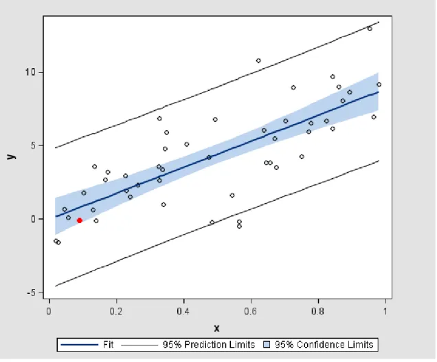
A scatter plot of these standard least squares prediction intervals for ysk is given in Figure

1.3.1. The target point xsk = 0.09207, corresponding to ysk= -0.19902,appears as a red

(13)

Table 1.3.1: Data

D = {(X

tj

,Y

tj

), t=1, …., 8; j=1, …, n

t,

=6}

ytj xtj 2.3414 0.26257 8.9471 0.72354 6.8076 0.49223 9.0282 0.85998 -0.1256 0.56269 6.525 0.77666 12.9706 0.95183 3.5447 0.67328 4.2364 0.47355 1.9865 0.22848 -0.1129 0.13894 3.5799 0.13257 2.9719 0.2258 4.2976 0.74852 8.6529 0.89218 3.8538 0.65574 5.9868 0.76902 3.6032 0.32458 -0.4854 0.56355 2.6332 0.32623 0.624 0.12862 -1.5436 0.02563 6.7194 0.70074 5.4871 0.6679 0.674 0.04329 9.7178 0.84142 3.3617 0.33593 6.8714 0.32671 -1.4588 0.0194 1.5276 0.23993 2.7107 0.16502 9.1589 0.98023 1.7803 0.10218 6.98 0.9628 3.8422 0.64433 6.0644 0.63606 6.2047 0.8407 0.113 0.05604 -0.2211 0.48219 6.7121 0.82239 3.2543 0.17164 5.1456 0.40807 5.9303 0.34821 1.6563 0.54267 4.8079 0.34307 1.0414 0.33842 8.0992 0.87013

(14)

Figure 1.3.1: A plot of the standard least squares prediction intervals for ysk

As will be explained later, first ignoring the block effect, we used the 95th percentile of an F distribution with 1 df in the numerator and 46 df in the denominator to construct an approximate 95% inverse prediction interval for xsk (method 1). Additionally, we

bootstrapped the distribution of T2 and used the 95th percentile of the bootstrapped distribution (F*) to form an approximate 95% inverse prediction interval for xsk (method

(15)

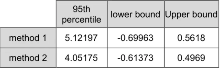
Table 1.3.2: Approximate 95% Inverse Prediction Intervals for xsk

_95th

percentile lower bound Upper bound method 1 5.12197 -0.69963 0.5618 method 2 4.05175 -0.61373 0.4969

Note that both intervals contain the value of xsk=0.092073 we are interested in predicting.

1.4: Organization of Remaining Chapters

In Chapter 2 we will show how we constructed approximate 1-α inverse prediction intervals for xsk with the methods used in the example above. Chapter 3 outlines the

simulation study that was used to compare the two methods. Chapter 4 explains the results of the simulation study, and Chapter 5 will summarize the findings of this report. Although many figures will be presented in the results chapter, for ease of reading it was necessary to place many of the tables and figures used to summarize our simulation results in appendices.

(16)

Chapter 2 – Inverse Prediction Interval

2.1: Background

The inverse prediction problem for a linear model with uncorrelated errors given by

2

1 , , ~ (0, ), 1, 2,..., ;

i o i i i

Y =β +βx +ε where ε N σ_ε i= n (2.1)

has been widely studied. See, for example, Brown (1979), Williams (1969), and Graybill (1976). Information on the robustness of these intervals may be found in Xiao (2000). However, to the best of my knowledge, the inverse prediction problem has not been studied in models with correlated errors. For the model with uncorrelated errors such as given in (2.1) above, Graybill (1976) developed a procedure for constructing an inverse prediction interval for a value xo having observed Y = yo.

2.2: Constructing an Inverse Prediction Set

We propose a method for constructing one-at-a-time interval estimates of the unobserved value x_sk corresponding to the observed value Y_sk =y_sk in the mixed model setting presented in section 1.1. This method closely follows Graybill’s procedure with a few adjustments. To illustrate, using equation (1.3), let

(

)

2 2 0 1 0 1 ˆ ˆ ( ) ˆ ˆ ˆ sk sk sk sk Y x F T Var Y x β β β β − − = = − − % (2.2)

Assume that F% is pivotal so that the quantiles of its distribution, denoted

{ }

F%_γ , are free of unknown parameters andx_sk. Recall that when there is no block effect and the

(17)

from an F distribution with 1 degree of freedom in the numerator and n-2 degrees of freedom in the denominator, where n=n1+n2+…+nt . Then, replacing all the entries in

(2.2) except x_sk by their observed values, a 1-α inverse prediction set,S for xsk is given

by

{

sk: 1

}

S = x F% ≤F%₋_α (2.3)

We proceed to solve for xsk by first noting that, after some simplification, the inequality

in (2.3) is equivalent to

(

Ysk−βˆ0−βˆ1xsk

)

2−Var Yˆ ( sk−βˆ0−βˆ1xsk)F%1−α ≤0 (2.4) where, 2 0 1 0 1 0 1 ˆ ˆ ˆ ˆ ˆ ˆ ˆ ˆ ₍ ₎ _ˆ _ˆ ˆ ₍ ₎ ˆ ₍ _{) 2} ₍ _, ₎ sk sk sk sk

Var Y −β −βx =σ_ε +σ_η +Var β +x Var β + x Cov β β

Combining terms, we obtain a quadratic equation that is a function of xsk

2 2 1 1 1 1 1 1 1 2 1 1 ˆ _{ˆ ( )}ˆ ₂ ˆ ˆ ˆ ₂ˆ ₍ ˆ _, ˆ₎ ˆ _ˆ _ˆ ˆ ˆ 2 ( ( ) 0 sk o sk o sk sk o sk Var F x Y Cov F x Y Y F Var α α α β β β β β β β β σ σ β − − − ε η  ₋  ₊  ₋ ₋        +_ − − + + _≤ % % % (2.5)

which can be expressed as ₍ ₎ 2 ₂ ₀

sk sk sk

q x =ax + bx + ≤c where a, b, and c are straightforwardly obtained from (2.5) and given by

2 1 1 1 ˆ _{ˆ ( )}ˆ ˆ ˆ ˆ ₂ˆ ₍ˆ _, ˆ₎ a Var F b Y Cov F α β β β β β β β − = − = − − % % (2.6)

(18)

The solutions to the quadratic equation obtained by setting the left hand side of (2.5) equal to zero can be one of the following:

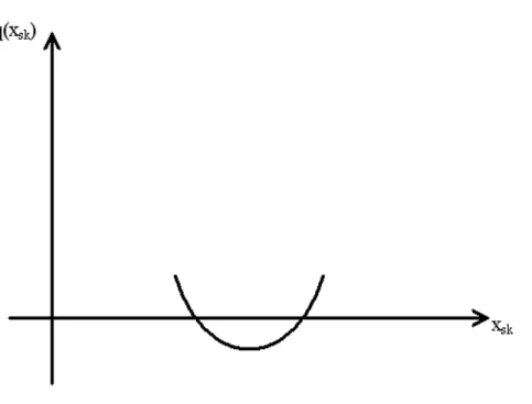
Case 1: a<0 and b²-ac<0: The resulting confidence interval is the whole real line.

Case 2: a<0 and b²-ac<0: b²-ac>0: the resulting confidence interval is the union of two semi-infinite pieces.

Case3: a>0 and b²-ac<0: the confidence interval does not exist.

Case4: a>0 and b²-ac>0: a confidence interval of finite length can be obtained.

We illustrate these cases with the subsequent figures:

(19)

Figure 2.2.2: Case 2: a<0, b²-ac>0

(20)

Figure 2.2.4: Case 4: a>0 and b²-ac>0

When there is no block effect, Graybill (1976) showed that Case 4 holds and a 1-α

confidence interval for xsk exists if and only if a>0, which is equivalent to rejecting the

hypothesis Ho: β1 = 0 in favor of Ha: β1 ≠ 0 with type I error rate α.. Graybill’s

algorithm, therefore, first carries out the test for zero slope and terminates without yielding a confidence interval for xsk if Ho is not rejected. The situation is more

complicated for the problem studied here where a block effect may exist, and ‘a>0’ does not guarantee that the discriminant, b²-ac, is positive. Nonetheless, the calibration problem is only meaningful if β1 ≠ 0 and we also use a two stage procedure where we

first test Ho: β1 = 0 vs. Ha: β1 ≠ 0. We use the asymptotic normality of REML estimators

and reject Ho with nominal type I error rate α if βˆ1 /se βˆ1 ≥zα/ 2. If Ho is rejected and b 2

-ac>0, we construct an inverse prediction interval for xsk with lower limit 2 ₄ , 2 b b ac a − − −

and upper limit

2 ₄

2

b b ac

a

− + −

. Method 1 will use the 1-α quantile

from an F distribution to evaluate a, b, and c. Method 2 will use the algorithm described below based on a bootstrap estimation of F% to evaluate a, b, and c.

(21)

2.3: Introduction to the Bootstrap

Using a bootstrap to approximate the distribution of a statistic is common practice. See for example Efron and Tibshirani (1998) where it is shown that an approximate

confidence interval for a parameter can be obtained by using the percentiles of the

bootstrap distribution of an appropriate pivotal. An assumption of the simple bootstrap is that the observations are independently and identically distributed. When this assumption holds, the bootstrap can be executed by sampling randomly with replacement from the observed data. Ideally, when bootstrapping the distribution of a pivotal, it is preferable to have a large number of bootstrap repetitions. Common practice is to carry out at least 1000 repetitions. Because of time limitations, in our study it was necessary to limit the number of bootstraps to 150.

2.4: Bootstrap Algorithm for Estimating F%_0.95

Suppose we have observed or generated data D = {(Xtj,Ytj), t=1, …., K; j=1, …, nt}

described in section 1.1 according to the algorithm given in section 3.3. And suppose we have rejected the hypothesis Ho: β1= 0 in favor of Ha:β1≠0 at nominal type I error rate.

Step 1*: Using a random number generator we simulated

{ }

(0, ˆ2)

tj iid N ε

ε∗ σ and

independently

{ }

η*_t iid N(0,σˆ_η2).

Step 1a*: Independently, also generate ˆ* ~ (0, ˆ2 ˆ2)

sk

e N σ_η +σ_ε and store for step 3b*

Step 2*: To create the bootstrap data we will use the errors we simulated in step 1* and the REML estimators β β σ σˆ₀, ˆ₁, ˆ_ε, ˆ_η to obtain data:

(22)

Step 3*: From data *

D using PROC MIXED of SAS we find estimators β β σ σˆ*₀, ˆ₁*, ˆ_ε*, ˆ_η*.

Step 3a*: We test Ho: ˆβ1=0. If Ho is rejected, go to 3b*. Otherwise, no interval is

obtained and return to bootstrap step 1*.

Step3b*: Using 1a*, estimate x_sk by

0 1 ˆ _ˆ ( ) ˆ ˆ sk sk sk y e x β β − − = (2.8) Step 4*: Compute * * * * * 0 1 ˆ _{ˆ ˆ} sk sk sk s Y = β + β x + ε +η (2.9)

Step 5*: Compute scaled *

F% to simplify the notation, we will denote this as F* given by

2 * * * * 0 1 * * * * 0 1 2 * * * 0 1 * * * 2 * * * 0 1 0 1 ˆ _{ˆ ˆ} 2 ˆ ₍ ˆ ˆ _ˆ ₎ ˆ _{ˆ ˆ} 2 _ˆ _ˆ ˆ ₍ ˆ ₎ _ˆ ˆ ₍ ˆ _{) 2}_ˆ ˆ ₍ˆ _, ˆ ₎ sk sk sk sk sk sk sk sk Y x n F n _{Var Y} _x Y x n

n _Var _{x Var} _{x Cov}

ε η β β β β β β σ σ β β β β   − −   = −  ₋ ₋      − −   =   − ₊ ₊ ₊ ₊   (2.10)

Independently steps 1-5 are repeated 150 times, yielding

{ }

* 150

1

j _j

F

= , which will then be

arranged in increasing order: * * * (1) (2) ... (150)

F ≤F ≤ ≤F . These order statistics can be used to approximate the 0.95 percentile of the distribution of F%

(23)

An approximate 0.95 inverse prediction interval for Xsk is then given by 2 4 4 2 b b ac a − ± − where 2 * 1 1 0.95 * 0 1 1 0 1 0.95 2 * 0 0.95 1 ˆ _{ˆ ( )}ˆ ˆ ˆ ˆ ₂ˆ ₍ˆ _, ˆ₎ ˆ _ˆ _ˆ ˆ ˆ 2 ( ( ) sk sk sk a Var f b Y Cov f c Y Y f _ε _η Var β β β β β β β β σ σ β = − = − − = − − + +

(24)

Equation Section (Next)

Chapter 3 – Simulation Study

3.1: Overview of Simulation Study

Our simulation investigates the performance of our two methods in constructing inverse confidence intervals. The investigation was carried out by simulating data that follow the model in equation (1.1) using a variety of settings. We then bootstrapped the distribution of F% using the algorithm described in section 3.4 and constructed approximate 95% inverse prediction intervals for xsk. using the 0.95 quantile of the bootstrapped distribution

and the 0.95 quantile of an F distribution. The performance of both methods was examined by measures such as coverage rate and average length of the confidence intervals. Our simulation was run in the statistical software SAS 9.1. Summary tables were made with Excel and figures of the results were made with the statistical software R as well as SAS 9.1.

3.2: Fitting the Model

The model from which we generated our data from can be expressed in matrix notation as

X

= +

Y

β

e, (3.1)

The way in which we generate the independent variables ensures that the design matrix X has full rank with probability 1 and e~N(0, V) where V=(etj), where etj is defined as in

(1.2). If we define ysk to be a new observation of the response Y, the covariance matrix K

is given by 2 2 ( , ) 0 t s J I for t s K Cov e e for t s η ε σ σ  ₊ ₌    = =  ≠     (3.2)

(25)

where J is a matrix of 1’s and I is the identity matrix, both having nt rows and nt

columns. Because we want to predict xsk given Y=ysk it was necessary to generate an xsk

so that we would have a way to compare our methods based on how the prediction intervals captured xsk. We chose to randomly generate xsk from a Uniform (0, 1)

distribution using the SAS RANUNI command.

3.3: Data Generation

Simulations were run in SAS using proc mixed for analysis and proc SQL for data

manipulation. SQL statements were needed in order to manipulate data properly, and join data sets together so that computations could be handled easier. Seed generation for each simulation was done using a random uniform number on (0, 1) and multiplying that number by1 10× 8, and truncating the result.

Steps used to generate data D.

Step 1: Generate ηt from N(0, ση), and independently {εtj} from N(0, σε). Step 2: Generate xtj from a Uniform(0,1) distribution.

Step 3: Let

Y_tj =β₀ +β₁x_tj +e_tj,

where

etj =

η

t+

ε

tj_.

(26)

Step 6: Compute 1 o sk sk sk Y =

β

+ x

β

+ e where, esk= ηs+ εsk

Step 7: Use PROC MIXED of SAS to estimate

β

_o ,

β

₁,σ , ε and ση _,store for later use.

Step 8: Test Ho:

β

₁=0, if Ho is rejected we will not form a confidence interval for that

replication of the simulation. We carry out the bootstrap only on the cases where Ho: β₁ =0 is rejected.

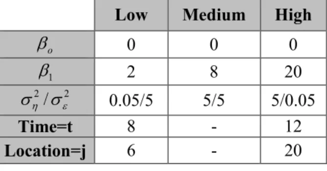
3.4: Simulation Settings

Simulation settings where chosen to see how coverage rates varied over different parameter values. Three different settings for β1 were chosen, these varied from low,

medium, and high. The parameter β0 was set to 0 for all simulations.

For the time variance, ση, and location variance, σ ,ε settings were chosen so that the

ratio of these quantities varied from low, medium and high. In the low ratio setting the location variance has a higher setting then the time variance. In the medium ratio setting, the ratio of the variances is equal. In the high ratio setting the time variance has a higher setting then the location variance. These settings were chosen in relation to the analysis of a split-plot design, and how well these tests perform due to the ratio of whole plot to sub plot error.

(27)

and the number of bootstraps per unique simulation setting had to be set in conjunction with the time and location settings so that a specific simulation could be completed in a reasonable amount of time. Thus settings for the factors time and location were chosen with only two levels, low and high. This was necessary to ensure that simulations would be able to be completed on time. A total of 36 different simulations were run. Below is a table with the settings discussed above:

Table 3.4.1: Parameter Settings

Low Medium High

o β 0 0 0 1 β 2 8 20 2 2 / η ε σ σ 0.05/5 5/5 5/0.05 Time=t 8 - 12 Location=j 6 - 20

Number of Bootstraps Replications: 150 Number of Replicated Simulations: 200

3.5: Simulation ID

In order to identify the different simulations a 5-digit character identifier was adopted for each simulation. The first digit represented the settings for the slope in our model: 1 = low (2), 2 = medium (8), and 3 = high (20). The second digit represented the settings for the ratio of the time variance to the location variance: 1=low (time .05/loc 5), 2=med (time 5/loc 5), and 3= high (time 5/loc .05). The third digit represented the amount of times in our model: 1=low (8), and 2=high (12). The fourth digit represented the amount of locations in our model: 1=low (6), and 2=high (20). The fifth digit was the value of the intercept and for this simulation study always had a default of zero.

(28)

An example of a simulation id would be: 12120. This id can be interpreted as having the following configuration: The first digit represents the slope and it has a value of 1 so the slope of our simulated model has been given the low setting (2). The second digit represents the ratio of time variance and location variance. The second digit has a value of 2 so the ratio of time variance over location variance has been given the medium setting (5/5). The third digits represents the number of times, it has a value of 1, which tells us that time has been given the low setting (8). The fourth digit represents the number of locations; and has a value of 2 so location has been given the high setting (20). The fifth digit represents the intercept, and for the purposes of this report will always be given the value of 0.

(29)

Chapter 4 - Results

4.1: Introduction to Results Chapter

We conducted a simulation study to compare the performance of the two methods described in section 1.1. These methods were used to obtain inverse prediction intervals for xsk in the mixed model setting given in equation (1.1). Evaluative measures such as

coverage rate, and average length and standard deviation of the interval lengths were used to compare the two methods. Additionally, McNemar’s test was carried out using PROC FREQ in SAS 9.1 to determine if the methods were performing the same for each distinct simulation setting. Tables of the simulation results used to create figures in sections 4.2, and 4.3 are in appendix B, and additional figures related to results described in section 4.2 are in appendix C. Each 2x2 table created using PROC FREQ and McNemar’s test can be found in appendix D.

Keep in mind that “Method 1” refers to the method that uses f0.95 , the 95th quantile of an

F distribution, to form approximate 95% inverse prediction sets for xsk, “Method 2” refers

to the method that uses * 0.95

f from the bootstrapped distribution of F%to form approximate 95% inverse prediction sets for xsk. The sections that follow will make use of the unique

simulation identifier denoted ‘simulation ID’ that was defined in section 3.5.

4.2: Average Interval Width and Standard deviation

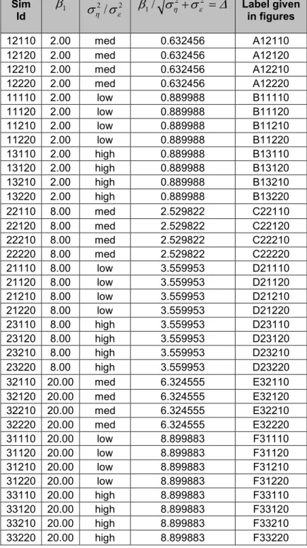
Using the table of data in appendix B, whisker plots were made for each unique

simulation and grouped byβ₁ settings (low=2, medium=8, high=20) and σ_η /σ_ε settings (low=0.05/5, medium=5/5, high=5/0.05). These figures are placed in Appendix D. The dot represents the mean length and whiskers extend to 1.96 times the standard error of the interval length, so that what are represented are 95% confidence intervals for the mean

(30)

The lengths for both methods are very large for the first twelve cases relative to the target valuesx_sk, which lies in the unit interval. Those 12 cases coincide with the 12

simulations whereβ₁ was set to low. Using the SAS procedure, PROC UNIVARIATE, a two-sided sign test was performed to compare mean interval length between method 1 and method 2 across the 36 separate simulation settings. The test yielded a p-value of 0.003 indicating that the mean lengths of the two methods are statistically significantly different.

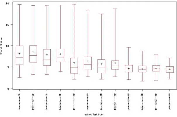
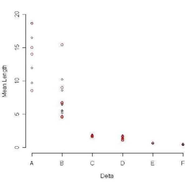
To further study interval length, Figures 4.2.1 – 4.2.4 present box plots of length plotted against an effect size type parameter ∆defined by

2 2

/ _η _ε

β σ σ

∆ = + (4.1)

For small ∆, observing ‘Y’ conveys little information about the corresponding ‘X’ and the test for zero slope is expected to have low power when ∆ > 0, unless sample size is large. The non-decreasing values of ∆in our design are given in the next to last column of table 4.2.1. All labels with same first letter, A-F, have the same ∆value. As expected, ignoring sample size, interval lengths for both methods decrease with increasing∆. The intervals are very wide for the first twelve cases, where ∆is smallest. Plots for both methods of mean length in figure 4.2.5 and median ‘mean length’ vs.∆ in figure 4.2.6 convey the same information. As in previous graphs where both methods were plotted red circles represent results based on method 1 and black circles represent results based on method 2. Note that in figure 4.2.5 and 4.2.6 it appears that mean length for method 2 tends to be higher than for method 1 for small values of ∆.

(31)

Table 4.2.1: Simulation ID with corresponding ∆ Sim Id 1 β 2_/ 2 η ε σ σ β1/ ση2+σε2 =∆ Label given in figures 12110 2.00 med 0.632456 A12110 12120 2.00 med 0.632456 A12120 12210 2.00 med 0.632456 A12210 12220 2.00 med 0.632456 A12220 11110 2.00 low 0.889988 B11110 11120 2.00 low 0.889988 B11120 11210 2.00 low 0.889988 B11210 11220 2.00 low 0.889988 B11220 13110 2.00 high 0.889988 B13110 13120 2.00 high 0.889988 B13120 13210 2.00 high 0.889988 B13210 13220 2.00 high 0.889988 B13220 22110 8.00 med 2.529822 C22110 22120 8.00 med 2.529822 C22120 22210 8.00 med 2.529822 C22210 22220 8.00 med 2.529822 C22220 21110 8.00 low 3.559953 D21110 21120 8.00 low 3.559953 D21120 21210 8.00 low 3.559953 D21210 21220 8.00 low 3.559953 D21220 23110 8.00 high 3.559953 D23110 23120 8.00 high 3.559953 D23120 23210 8.00 high 3.559953 D23210 23220 8.00 high 3.559953 D23220 32110 20.00 med 6.324555 E32110 32120 20.00 med 6.324555 E32120 32210 20.00 med 6.324555 E32210 32220 20.00 med 6.324555 E32220 31110 20.00 low 8.899883 F31110 31120 20.00 low 8.899883 F31120 31210 20.00 low 8.899883 F31210 31220 20.00 low 8.899883 F31220 33110 20.00 high 8.899883 F33110 33120 20.00 high 8.899883 F33120 33210 20.00 high 8.899883 F33210 33220 20.00 high 8.899883 F33220

(32)

Figure 4.2.1: Box plots of method 1 interval lengths vs. ∆ (A-B)

(33)

Figure 4.2.3: Box plots of method 1 interval lengths vs. ∆ (C-F)

(34)

(35)

(36)

4.3: Coverage Rate

Table (4.3.1) presents estimated coverage rates of nominal 0.95 confidence intervals for

sk

x based on those data sets for which intervals could be constructed. The standard errors of these estimates vary among the Simulation ID’s since the number of sets where S is an interval varies among the parameter settings (see section 4.4). As a rough guide,

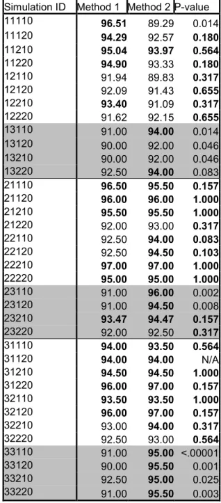
(.89)(.11) /100=0.031provides an approximate upper bound on these standard errors. Cases where a 95% confidence interval for coverage rate contains the target rate of ‘0.95’ are indicated in bold. Method 2 appears to have more simulations where the coverage rate is captured by the 0.95 confidence interval then does method 1. However, overall both methods appear to have coverage rates below nominal for about 1/3 of the simulation settings.

McNemar’s test for the equality of two correlated proportions was used to test for a difference between the coverage rates across the cases that were investigated. The estimated rates are correlated since both methods were used on the same data set

generated under each setting. P-values from McNemar’s test are given in Table (4.4.1). From this table we see that with the exception of a few simulations, the simulations where McNemar’s test found a significant difference between the two methods are those where the variance ratio is set to high. This signifies that the performance of the two methods is significantly different in terms of coverage rate as long as the time variance component is large relative to the location variance component.

(37)

Table 4.4.1: Simulation coverage rates for method 1 and method 2

Simulation ID Method 1 Method 2 P-value 11110 _96.51 _89.29 _0.014 11120 94.29 92.57 0.180 11210 95.04 93.97 0.564 11220 94.90 93.33 0.180 12110 91.94 89.83 0.317 12120 92.09 91.43 0.655 12210 93.40 91.09 0.317 12220 91.62 92.15 0.655 13110 _91.00 94.00 0.014 13120 _90.00 _92.00 _0.046 13210 90.00 92.00 0.046 13220 92.50 94.00 0.083 21110 96.50 95.50 0.157 21120 96.00 96.00 1.000 21210 95.50 95.50 1.000 21220 92.00 93.00 0.317 22110 92.50 94.00 0.083 22120 92.50 94.50 0.103 22210 97.00 97.00 1.000 22220 95.00 95.00 1.000 23110 91.00 96.00 0.002 23120 91.00 94.50 0.008 23210 93.47 94.47 0.157 23220 92.00 92.50 0.317 31110 94.00 93.50 0.564 31120 94.00 94.00 N/A 31210 94.50 94.50 1.000 31220 96.00 97.00 0.157 32110 93.50 93.50 1.000 32120 96.00 97.00 0.157 32210 93.00 94.00 0.317 32220 92.50 93.00 0.564 33110 91.00 95.00 <.00001 33120 90.00 95.50 0.001 33210 92.50 95.00 0.025 33220 _91.00 _95.50 _0.003

(38)

Figure 4.4.1 plots the coverage rates for the two methods given in Table 4.4.1 against one another. Here, we see little relation between the rates for the two methods.

Figure 4.4.1: Plot of coverage rate for method 1 vs. coverage rate for method 2

Coverage rates for both methods are plotted against the slope β₁ in Figure 4.4.2 against variance ratio in Figure 4.4.3, against time in Figure 4.4.4 and against location in Figure 4.4.5. Black Circles Represent results based on method 2 and red circles represent results

(39)

higher coverage rate then method 2 when the slope (β₁) is set to low (2), and method 2 appears to have a higher coverage rate then does method 1 when the variance ratio (σ_η2/σ_ε2) is high (5/0.05).

(40)

(41)

(42)

(43)

Figure 4.4.6 plots coverage rate vs. mean length. There appears to be a slight downward trend in coverage rate as mean length increases, but this could be due to the low slope setting for those simulations and the resulting smaller number of confidence intervals that could be constructed due to the slope being zero. Other then this there appears to be little relation between these variables for both methods.

(44)

4.4: Bootstrap Diagnostics

Although the number of bootstraps used to approximate the distribution of F% was fixed to be 150, not every bootstrap was able to be carried to the final step. If the condition

1

ˆ ₀

β ≠ from Step 3a*in Section 2.4 was not met, f* could not be computed. To determine, on average, how many f*’s were actually involved in approximating the

distribution of F%for each unique simulation setting, the following measure was adopted.

Consider a given simulation setting, and a single inverse prediction interval i, i=1,…,200, within that setting. For that given simulation, and inverse prediction interval i, denote the number of bootstraps where βˆ₁≠0 by Mi. The table below summarizes the average

number of M si' , denoted M,and standard deviation of the M si' , denoted SM, for each

(45)

Table 4.3.1: M S, M Simulation ID _M s_M 11110 69.59 44.9697 11120 121.995 32.9077 11210 87.225 46.1277 11220 138.52 19.9136 12110 91.85 43.3037 12120 118.66 33.8763 12210 79.07 44.4412 12220 137.18 23.0223 13110 149.955 0.2307 13120 150 0 13210 149.935 0.2667 13220 150 0 21110 149.535 5.6059 21120 150 0 21210 150 0 21220 150 0 22110 149.77 0.8723 22120 150 0 22210 149.99 0.0997 22220 150 0 23110 149.935 0.2471 23120 150 0 23210 149.905 0.3113 23220 150 0 31110 150 0 31120 150 0 31210 150 0 31220 150 0 32110 150 0 32120 150 0 32210 150 0 32220 150 0 33110 149.975 0.1565 33120 150 0 33210 149.965 0.1842 33220 150 0

Note that most of the bootstraps whereHo :β1 =0 was not rejected were those where the slope,β₁ was set to low and the variance ratio was at the low and medium settings.

(46)

4.5: Simulation Diagnostics

Recall that both methods first testH₀:β₁ =0and check to see if the discriminate is positive before attempting to construct a confidence interval forx_sk.Table (5.3.1) indicates that both methods fail at high rates to yield intervals when β1 is at its low

setting. This agrees with what we found in Table (4.3.1) when we summarized for which simulations ˆβ₁ ≠0 Additionally Table (4.4.1) shows that Method 1 did not have any intervals where the discriminant was negative, but Method 2 did give some confidence intervals where the discriminant was negative in spite of the fact that the slope was found to be nonzero for those intervals.

Table 4.4.1: Settings for which β1=0 or b2-ac<0

Sim Id Total number of intervals that could not be formed Method 1 Total number of intervals that could not be formed Method 2 Intervals where slope non-zero, but b^2-ac<0 Method 1 Intervals where slope non-zero, but b^2-ac<0 Method 2 Intervals where Slope is 0 11110 114 116 0 2 114 11120 25 25 0 0 25 11210 79 84 0 5 79 11220 4 5 0 1 4 12110 76 82 0 6 76 12120 23 25 0 2 23 12210 94 99 0 5 94 12220 9 9 0 0 9 23210 1 1 0 0 1

(47)

Chapter 5 - Summary and Conclusion

This report proposed and studied a solution to the calibration or inverse prediction problem in a mixed model setting where experimental units were selected from blocks that are treated as random effects. Two methods for producing inverse prediction

intervals for xsk were compared. Method 1 made inverse prediction intervals in the same

way as Graybill proposed for the simple linear model by using quantiles from an F distribution. Method 2 accounts for the block effect by using a bootstrap to approximate the distribution of F% _{and forms inverse prediction intervals for x}sk with quantiles from

the bootstrapped distribution of F%._{While results from each method indicate that both}

methods maintain coverage rates below 0.95 for approximately 1/3 of the chosen simulation settings. method 2 appears to have a slightly better coverage rate then does method 1.

Overall, method 2 produced coverage rates for prediction intervals near ninety-five percent. Thus within the space of our parameter settings, one might prefer method 2 over method 1. However when the slope setting is set to low, we notice some problems with method 2’s approach. Specifically, some prediction intervals fail to form due to the discriminate being negative. In this case method 1 is a better choice since this procedure never failed to yield an interval where the discriminate was negative. Other problems such as computer resources may limit the use of method 2, since the bootstrap algorithm used to produce the intervals must be performed on a machine with good resources, namely a fast processor. For a researcher with limited resources and time, method 1 might be the best choice; especially since the coverage rate of intervals constructed using method 1 is comparable to the coverage rate of intervals constructed using method 2. One must also take into consideration that method 1 makes a strong assumption by using a statistic from an F distribution, thus one can see the utility of method 2. While the author of this paper would recommend method 2 with some restrictions as stated, further

(48)

Additionally, investigation should be carried out into why, for certain settings, Method 2 produced intervals that could not be formed due to the discriminant being negative. Also, other simulations should be carried out with added settings for all the parameters, in particular the settings for number of locations and times, and the variance ratio. Limited resources were available for running our simulations, and thus settings had to be chosen accordingly. However, in a high performance computing environment (HPC) one could take advantage of clusters and run very fast simulations with additional settings for all parameters as well as higher location and time settings. The availability of HPC would give us a better understanding of the behavior of both methods, and might lead to a better theoretical understanding behind the performance the two methods.

(49)

References

Casella, G. and Berger, R. L. (1990). Statistical Inference. Wadsworth/Brooks Cole, Pacific Grove, CA.

Brown, G.H. (1979). An optimisation criterion for linear inverse estimation.

Technometrics 21, 575-579.

Efron, B. (1979). Bootstrap methods: Another look at the jackknife. Ann. Statist. 7, 1- 26.

Efron, B and Tibshirani, R. (1998). An Introduction to the Bootstrap (Monographs on Statistics and Applied Probability). CRC Press LLC, Boca Raton, FL.

Jiang, J. (1996). REML estimation: Asymptotic behavior and related topics. Ann. Statist. 24, 255-286.

Graybill, F.A. (1976). Theory and Application of the Linear Model. Duxbury, United States.

Shukla. G.K. (1972). On the problem of calibration. Technometrics, 14:547-553.

Williams, E.J. (1969a). Regression methods in calibration problems. BUN. Int. Statbt. Inst. 43, 17-28.

Williams, E.J. (1969b). A note on regression methods in calibration. Technometrics 11,

189-192.

(50)

APPENDIX A – SIMULATION CODE

The following is the simulation code I ran for my report. Following this is additional code I used to merge information from all simulations together, and perform additional

analyses that were required.

/********************************************************************** Version history Documentation:

04-01-07 Beginning step 1 and 2 have been verified. Verification:

Steps 3 and 4, must be properly verified by hand. Future/Current issues:

*Data clean up, clean up data not needed/or used during process.

*variance formula needs to be computed from proposal. *need to asses how SAS determines arbitrary

percentiles from a data sample.

*Denominator 0 issue will need to be adressed. *Optimize sql statements IF needed.

06-04-07s

Verification:

Code had been verified. Future/Current issues:

Generating multiple real experiments is taken care of.

See above. 06-13-07

Future issues:

Made good progress but now optimization is an issue SQL,

12-26-07

Verification:

Have checked program for errors.All the data sets are producing what is desired.

*********************************************************************** ********************/

/*time v and loc v represent the variances for time and location in the "real" experiment*/

%macro do_simulation(

seed, alpha,

(51)

num_l, intercept, slope, var_terror, var_lerror, num_stat, num_reps, ID);

libname storage 'C:\test_case'; run;

libname output 'C:\test_case'; run;

PROC PRINTTO LOG="c:\logfile.log"; run;

proc printto print="c:\output.out"; run;

%let seed_increment=1; run;

/****************************************************/ /* This is the real life data set that we are using */ /* This will contain the estimated b_0 and b_1 */

data real_Dset; good_b1hat=0; do rep=1 to &num_reps; x_sk=ranuni(&seed); time_sk=sqrt(&var_terror)*rannor(&seed); loc_sk=sqrt(&var_lerror)*rannor(&seed); do t=1 to &num_t; time_error = 0+sqrt(&var_terror)*rannor(&seed); do j=1 to &num_l; location_error = 0+sqrt(&var_lerror)*rannor(&seed); x=ranuni(&seed); bo=&intercept; b1=&slope; y=bo+b1*x+time_error+location_error; y_sk=bo+b1*x_sk+time_sk+loc_sk; output; end; end; end;

DROP time_sk loc_sk; run;

(52)

/* Analyze the data set real_dset marking those ones with good=1 and good=0 */

DM 'Log; Clear;output;clear;'; run;

ods exclude all;

proc mixed data=real_dset CL method=REML; by rep;

class t j;

model y=x / cl ddfm=kr solution CovB; random t;

ods output covparms=var_params CovB=Cov_fix solutionf=solution_fixed tests3=type3test;

run;

ods exclude none;

/* Note that this step is redundant but it's an extra check.

One should not see a good value of 0 anymore! Examine type3test below if worried about it.

*/

data type3test; set type3test; good_b1hat=0;

if probf<=.05 then good_b1hat=1; run;

data solution_fixed; set solution_fixed;

if effect="Intercept" then effect="B_0hat"; if effect="x" then effect="B_1hat";

run;

data var_params; set var_params;

if covparm="t" then covparm="time_v";

if covparm="Residual" then covparm="loc_v"; run;

/********************************************************************** ***********************/

/* Finding the covariance between B_0hat and B_1hat, finding the variance of B_1hat

finding the variance of B_0hat*/

proc sql;

create table data_prep8a as select

(53)

rep from cov_fix where row=1; quit;

proc sql;

create table data_prep8b as select col2 as var_b1hat, rep from cov_fix where row=2; quit; proc sql;

create table data_prep8c as select a.*,

b.*

from data_prep8a as a, data_prep8b as b where a.rep=b.rep;

proc transpose data=solution_fixed out=solution_fixed2; by rep;

ID Effect; run;

proc transpose data=var_params out=var_parms2; by rep;

ID covparm; run;

/******* End real data set *****/

/******** Begin step 1 ***********/ data step1; do rep=1 to &num_reps; do exp=1 to &num_stat; do t=1 to &num_t; time_error_star = 0+rannor(&seed); do j=1 to &num_l; location_error_star =0+rannor(&seed); output; end; end; end; end;

(54)

create table temp_step as select distinct

a.*,

b.time_v, b.loc_v

from step1 as a, var_parms2 as b where a.rep=b.rep AND b._name_="Estimate"; quit; data step1; set temp_step; time_error_star=time_error_star*sqrt(time_v); location_error_star=location_error_star*sqrt(loc_v); DROP time_v loc_v;

run;

proc sql;

create table step1a as select a.*, b.x, b.x_sk, b.y_sk, c.B_0hat, c.B_1hat, d.time_v, d.loc_v, e.good_B1hat

from step1 as a, real_dset as b, solution_fixed2 as c,var_parms2 as d, type3test as e

where a.t=b.t AND a.j=b.j AND c._name_="Estimate"

AND d._name_="Estimate" AND a.rep=b.rep

AND a.rep=c.rep and a.rep=d.rep and a.rep=e.rep; quit;

proc sort data=step1a; by rep exp;

run;

proc datasets library=work;

delete solution_fixed2 var_parms2 step1 temp_step; run;

(55)

/* Step 2 needed no modification for multiple intervals */ /********************************************************/

data dstar; set step1a;

y_star=B_0hat+B_1hat*x+time_error_star+location_error_star; good_b1hatstar=0; /* again for generate macro below */

run;

proc datasets library=work; delete step1a;

run;

/* This finishes step2 */

/******************************************************************/ /** STEP 3

/*

/******************************************************************/

DM "Log; Clear; output; clear"; run;

ods exclude all;

proc mixed data=dstar CL method=REML; by rep exp;

class t j;

model y_star=x / cl ddfm=kr solution CovB; random t;

ods output covparms=var_params_star CovB=Cov_fixstar solutionf=solution_fixed_star tests3=type3test; run;

ods exclude none;

data type3test; set type3test; good_b1hatstar=0;

if probf<=.05 then good_b1hatstar=1; run;

(56)

run;

data var_params_star; set var_params_star;

if covparm="t" then covparm="time_vhatstar";

if covparm="Residual" then covparm="loc_vhatstar"; run;

proc transpose data=solution_fixed_star out=solution_fixed_star2; by rep exp;

ID Effect; run;

proc transpose data=var_params_star out=var_params_star2; by rep exp;

ID covparm; run;

proc sql;

create table step3a as select a.*, c.B_0hatsta as B_0hatstar, c.B_1hatsta as B_1hatstar, d.time_vhat as time_vhatstar, d.loc_vhats as loc_vhatstar, e.good_b1hatstar as testing_b1hatstar

from dstar as a, solution_fixed_star2 as c,var_params_star2 as d, type3test as e

where a.exp=c.exp AND a.exp=d.exp AND a.exp=e.exp AND

a.rep=c.rep AND a.rep=d.rep AND a.rep=e.rep AND c._name_="Estimate"

AND d._name_="Estimate"; quit; data step3a; set step3a; testing_b1hat=good_b1hat; drop good_b1hat; run;

/* Must generate the x_skhats */ data step3temp; do rep=1 to &num_reps; do exp=1 to &num_stat; x_skhat=0; e_skhat_source = rannor(&seed+9);

(57)

loc_error_source=rannor(&seed+9);

/* These should be in step 4 but it runs easier */

do t=1 to &num_t; do j=1 to &num_l; output; END; END; END; END; run; proc sql;

create table step3b as select a.*, b.x_skhat, b.e_skhat_source, b.time_error_source, b.loc_error_source from step3temp as b, step3a as a where a.rep=b.rep AND a.exp=b.exp AND a.t=b.t AND a.j=b.j; quit; data step3; set step3b; if testing_b1hat = 1 then x_skhat=(y_sk-B_0hat-(sqrt(time_v)*e_skhat_source+sqrt(loc_v)*e_skhat_source))/B_1hat; else x_skhat = .; run;

delete step3temp step3a step3b dstar; run;

/**********/ /* Step 4 */ /**********/ /*

For naming conventions I use the _sk to denote a subscript of sk, the star suffixed at the end means a stared notation variable, thus: y_skstar = a variable y with sk subscript that is superscripted with star.

While this sounds complex, it clearly explains the intended usage of this variable in our work.*/

(58)

timeerror_skstar=sqrt(time_v)*time_error_source; locerror_skstar=sqrt(loc_v)*loc_error_source;

y_skstar=b_0hat+b_1hat*x_skhat+timeerror_skstar+locerror_skstar; drop time_error_source loc_error_source;

run;

proc datasets library=work; delete step3; run; quit; /*************************************/ /* End of step 4 */ /*************************************/ /*** Begin step 5 ***/ proc sql;

create table step5a as select exp, rep, col1 as var_b0hatstar, col2 as cov_b1b0hatstar from cov_fixstar where row=1

order by rep, exp; quit;

proc sql;

create table step5b as select exp, rep, col2 as var_b1hatstar from cov_fixstar where row=2

order by rep, exp; quit;

proc sql;

create table step5c as select a.*,

b.*

from step5a as a, step5b as b where a.exp=b.exp and a.rep=b.rep; quit;

(59)

select a.*, b.*

from step5c as a, step4 as b where a.exp=b.exp and a.rep=b.rep; run; data step5; set step5d; num_t=&num_t; num_l=&num_l;

scale = (num_t*num_l) / ( (num_t*num_l) - 2 ) ; top=y_skstar-B_0hatstar-(B_1hatstar*x_skhat);

bottom=sqrt(time_vhatstar+loc_vhatstar+var_b0hatstar+((x_skhat*x_skhat) *var_b1hatstar)+2*(x_skhat*cov_b1b0hatstar));

F_star=(scale)*((top/bottom)**2); drop num_t num_l scale;

run; proc sql;

create table storage.counting_mi_&ID as select distinct exp, rep, testing_b1hat, testing_b1hatstar from step5; quit;

delete step5a step5b step5c step5d step4; quit;

/**** Step 6 is already completed. ****/ /* step7 */

proc sort data=step5 out=step7 NODUPKEY;

where testing_b1hat=1 and testing_b1hatstar=1; by rep exp f_star;

(60)

by rep;

var F_star;

output out=percentiles pctlpts=95 pctlpre=P; run;

/****************** STEP 8 *************************/

/* Computing the confidence intervals */

/***************************************************/

data step8a; set percentiles; f1=p95;

run;

/* First grab the data needed from tables lying about */

proc sql;

create table step8b as select distinct c.f1, a.b_1hat, a.b_0hat, a.testing_b1hat, b.var_b1hat, b.var_b0hat, a.y_sk, b.cov_b1b0hat, a.time_v, a.loc_v, a.x_sk, a.rep from step7 as a, data_prep8c as b, step8a as c where c.rep=a.rep AND c.rep=b.rep AND testing_b1hat=1 order by rep; quit; data quadratic_coefficients; set step8b; a = (b_1hat**2)-(var_b1hat*f1); b = ((b_0hat*b_1hat)-(b_1hat*y_sk)-(cov_b1b0hat*f1));

c = (y_sk**2)-2*(b_0hat*y_sk)+(b_0hat**2)-f1*(time_v+loc_v+var_b0hat); run;

data storage.quadratic_coefficients_&ID; set quadratic_coefficients;

run;

(61)

run;

/* finally the confidence interval */

data step8(KEEP=a b c lower upper rep x_sk p_score); set quadratic_coefficients;

lower=(-2*b-sqrt((4*b**2)-4*a*c))/(2*a); upper=(-2*b+sqrt((4*b**2)-4*a*c))/(2*a);

if (x_sk>=lower) AND (x_sk<= upper) AND (lower^=.) AND (upper^=.) then p_score=1;

else if lower=. AND upper=. then p_score=-1; else p_score=0;

run;

proc sql;

create table p_valinformation as select count(*) as total,

sum(p_score) as successes from step8 where

p_score^=-1; quit; data p_valinformation; set p_valinformation; coverage=successes/total; run;

/* At the end of the simulation now need to count up proper scores 1. Count the number of times proc mixed grabbed the true value of B_1hat B_0hat and

time error and location error hats. 2. Same for Stars.

3. Coverage rate for x_sk 4. Mean length of intervals

5. Number of runs actually computed. */

/* For this table our rates of estimation only care about where B_1hat was estimated to not be 0.

*/

/* This is used as a reference table for calculations */ /* First part is to tally the parameter estimates */

/* Begin with only checking those experiments that have B_1hat being non-zero.

This is done by establishing a reference table that tells you what the good real

(62)

testing_b1hat, rep from step5 where testing_b1hat=1; quit; proc sql;

create table b0b1_checking as select a.*

from solution_fixed as a, good_reference as b where

a.rep=b.rep; quit;

proc sql;

create table time_loc_varchecking as select a.*

from var_params as a, good_reference as b where a.rep=b.rep; quit; data b0b1_checking; set b0b1_checking; intercept_score=0;

if &intercept>= lower AND &intercept<=upper then intercept_score=1;

slope_score=0;

if &slope>= lower and &slope<=upper then slope_score=1; run;

data time_loc_varchecking; set time_loc_varchecking; time_score=0;

if &var_terror >= lower AND &var_terror <= upper then time_score=1;

loc_score=0;

if &var_lerror >= lower AND &var_lerror <= upper then loc_score=1;

run;

proc summary data=b0b1_checking; class effect;

var intercept_score slope_score; output out=b0b1_score sum=; run;

proc summary data=time_loc_varchecking; class covparm;

var time_score loc_score; output out=timeloc_score sum=;

(63)

/* Now to do the same with the star sets */

/* Must form a reference table again, I only want to check those that had B_1hat being not 0, and B_1hatstar being not 0

*/

proc sql;

create table good_reference_star as select distinct a.rep, a.exp, a.testing_b1hat, a.testing_b1hatstar from step5 as a where a.testing_b1hat=1 AND a.testing_b1hatstar=1; quit; proc sql;

create table b0b1star_checking as select a.*

from solution_fixed_star as a, good_reference_star as b where

a.rep=b.rep AND a.exp=b.exp; quit;

proc sql;

create table timestar_locstar_varchecking as select a.*

from var_params_star as a, good_reference_star as b where a.rep=b.rep AND a.exp=b.exp; quit; data b0b1star_checking; set b0b1star_checking; intercept_score=0;

if &intercept>= lower AND &intercept<=upper then intercept_score=1;

slope_score=0;

if &slope>= lower and &slope<=upper then slope_score=1; run;

data timestar_locstar_varchecking; set timestar_locstar_varchecking;

(64)

loc_score=0;

if &var_lerror >= lower AND &var_lerror <= upper then loc_score=1;

run;

proc summary data=b0b1star_checking; class effect;

var intercept_score slope_score; output out=b0b1star_score sum=; run;

proc summary data=timestar_locstar_varchecking; class covparm;

var time_score loc_score;

output out=timelocstar_score sum=; run;

/* Now we need to put this data set together */

/* Grab data from the score tables and put it into variables */

proc sql;

select intercept_score into :b0_hatscores from b0b1_score

where effect="B_0hat"; quit;

proc sql;

select slope_score into :b1_hatscores from b0b1_score

where effect="B_1hat"; quit;

proc sql;

select time_score into :time_varscores from timeloc_score

where covparm="time_v"; quit;

proc sql;

select loc_score into :loc_varscores from timeloc_score

where covparm="loc_v"; quit;

proc sql;

select _freq_ into :good_b1hats from b0b1_score

(65)

/* Now we adress stars */

proc sql;

select intercept_score into :b0star_hatscores from b0b1star_score

where effect="B_0hatsta"; quit;

proc sql;

select slope_score into :b1star_hatscores from b0b1star_score

proc sql;

select time_score into :timestar_varscores from timelocstar_score

where covparm="time_vhat"; quit;

proc sql;

select loc_score into :locstar_varscores from timelocstar_score

where covparm="loc_vhats"; quit;

proc sql;

select _freq_ into :good_b1hatsandstars from b0b1star_score

/* Now need to do calculations for statistics based on the confidence intervals:

1. Get the mean length.

2. Count the number of good ones

3. Give the numbers for a coverage rate. */

/* define the length of a CI as abs(upper-lower) */

data step8; set step8;

length=abs(upper-lower); run;

/* Now use proc means to obtain the length where the CS is valid: p_score=1 or p_score=0

(66)

run;

/* The data set P_valinformation has all the information about coverage for 2. */

proc sql;

select averagelength into :average_ci_length from cilengths;

quit; proc sql;

select coverage into :ci_coverage from p_valinformation;

select successes into :ci_goodcount from p_valinformation;

select total into :total_cis from p_valinformation;

quit;

/* Final report datasets */

data storage.final_report_&ID; b0=&b0_hatscores; b1=&b1_hatscores; timev=&time_varscores; locv=&loc_varscores; b1_hatcount=&good_b1hats; b0_star=&b0star_hatscores; b1_star=&b1star_hatscores; timev_star=&timestar_varscores; locv_star=&locstar_varscores; b1_hatstarcount=&good_b1hatsandstars; Total_possible_b1hats=&num_reps;

Total_possible_b1hatstars=%eval(&num_reps*&num_stat); average_length=&average_ci_length; x_skci_successes=&ci_goodcount; x_skci_total=&total_cis; coverage=&ci_coverage; bad_cis=Total_possible_b1hats-x_skci_total; run; proc sql;

create table diagnostic_&id as select distinct

rep, exp,

testing_b1hat, testing_b1hatstar