©2005 Hindawi Publishing Corporation RESEARCH ARTICLE
Gene Expression Data Classification With Kernel
Principal Component Analysis
Zhenqiu Liu,1 Dechang Chen,2 and Halima Bensmail3 1Bioinformatics Cell, US Army Medical Research and Materiel Command,
110 North Market Street, Frederick, MD 21703, USA
2Department of Preventive Medicine and Biometrics, Uniformed Services University of the Health Sciences,
4301 Jones Bridge Road, Bethesda, MD 20814, USA
3Department of Statistics, University of Tennessee, 331 Stokely Management Center, Knoxville, TN 37996, USA
Received 3 June 2004; revised 28 August 2004; accepted 3 September 2004
One important feature of the gene expression data is that the number of genesMfar exceeds the number of samplesN. Standard statistical methods do not work well whenN < M. Development of new methodologies or modification of existing methodologies is needed for the analysis of the microarray data. In this paper, we propose a novel analysis procedure for classifying the gene expression data. This procedure involves dimension reduction using kernel principal component analysis (KPCA) and classification with logistic regression (discrimination). KPCA is a generalization and nonlinear version of principal component analysis. The proposed algorithm was applied to five different gene expression datasets involving human tumor samples. Comparison with other popular classification methods such as support vector machines and neural networks shows that our algorithm is very promising in classifying gene expression data.
INTRODUCTION
One important application of gene expression data is the classification of samples into different categories, such as the types of tumor. Gene expression data are charac-terized by many variables on only a few observations. It has been observed that although there are thousands of genes for each observation, a few underlying gene compo-nents may account for much of the data variation. Prin-cipal component analysis (PCA) provides an efficient way to find these underlying gene components and reduce the input dimensions (Bicciato et al [1]). This linear transfor-mation has been widely used in gene expression data anal-ysis and compression (Bicciato et al [1], Yeung and Ruzzo [2]). If the data are concentrated in a linear subspace, PCA provides a way to compress data and simplify the repre-sentation without losing much information. However, if the data are concentrated in a nonlinear subspace, PCA
Correspondence and reprint requests to Zhenqiu Liu Bioin-formatics Cell, U.S. Army Medical Research and Materiel Command, 110 North Market Street, Frederick, MD 21703, USA, E-mail: [email protected]
This is an open access article distributed under the Creative Commons Attribution License which permits unrestricted use, distribution, and reproduction in any medium, provided the original work is properly cited.
will fail to work well. In this case, one may need to con-sider kernal principal component analysis (KPCA) (Rosi-pal and Trejo [3]). KPCA is a nonlinear version of PCA. It has been studied intensively in the last several years in the field of machine learning and has claimed success in many applications (Ng et al [4]). In this paper, we intro-duce a novel algorithm of classification, based on KPCA. Computational results show that our algorithm is effective in classifying gene expression data.
ALGORITHM
A gene expression dataset withMgenes (features) and
NmRNA samples (observations) can be conveniently rep-resented by the following gene expression matrix:
X= x11 x12 · · · x1N x21 x22 · · · x2N .. . ... . .. ... xM1 xM2 · · · xMN , (1)
where xli is the measurement of the expression level of genelin mRNA samplei. Letxi =(x1i, x2i, . . . , xMi)
de-note theith column (sample) ofXwith the prime repre-senting the transpose operation, andyithe corresponding class label (eg, tumor type or clinical outcome).
KPCA is a nonlinear version of PCA. To perform KPCA, one first transforms the input data x from the
original input spaceF0into a higher-dimensional feature
spaceF1with the nonlinear transformx→Φ(x), whereΦ
is a nonlinear function. Then a kernel matrixKis formed using the inner products of new feature vectors. Finally, a PCA is performed on the centralizedK, which is the es-timate of the covariance matrix of the new feature vector inF1. Such a linear PCA onKmay be viewed as a
nonlin-ear PCA on the original data. This property is sometimes called “kernel trick” in the literature. The concept of ker-nel is very important, here is a simple example to illustrate it. Suppose we have a two-dimensional inputx=(x1, x2),
let the nonlinear transform be
x−→Φ(x)=x2 1, x22, √ 2x1x2, √ 2x1, √ 2x2,1 . (2) Therefore, given two pointsxi=(xi1, xi2)andxj=(xj1,
xj2), the inner product (kernel) is
Kxi,xj=ΦxiΦxj =x2 i1x2j1+xi22x2j2+ 2xi1xi2xj1xj2 + 2xi1xj1+ 2xi2xj2+ 1 =1 +xi1xj1+xi2xj2 2 =1 +xixj2, (3)
which is a second-order polynomial kernel. Equation (3) clearly shows that the kernel function is an inner product in the feature space and the inner products can be evalu-ated without even explicitly constructing the feature vec-torΦ(x).
The following are among the popular kernel func-tions:
(i) first norm exponential kernel
Kxi,xj=exp−β xi−xj , (4) (ii) radial basis function (RBF) kernel
Kxi,xj=exp −xi−xj 2 σ2 , (5)
(iii) power exponential kernel (a generalization of RBF kernel) Kxi,xj=exp − xi−xj 2 r2 β , (6)
(iv) sigmoid kernel
Kxi,xj=tanhβxixj, (7) (v) polynomial kernel
Kxi,xj=xixj+p2
p1,
(8) wherep1andp2=0,1,2,3, . . .are both integers.
For binary classification, our algorithm, based on KPCA, is stated as follows.
KPC classification algorithm
Given a training dataset {xi}ni=1 with class labels
{yi}ni=1and a test dataset{xt}ntt=1 with labels {yt}ntt=1, do
the following.
(1) Compute the kernel matrix, for the training data,
K =[Kij]n×n, whereKij =K(xi,xj). Compute the kernel matrix, for the test data, Kte = [Kti]nt×n, whereKti = K(xt,xi).Kti projects the test dataxt onto training dataxiin the high-dimensional fea-ture space in terms of the inner product.
(2) CentralizeKusing andKte
K= In−n11n1n KIn−1n1n1n , Kte= Kte− 1 n1nt1nK I−1 n1n1n . (9)
(3) Form ann×kmatrixZ=[z1 z2 · · · zk], where
z1, z2, . . . , zk are eigenvectors ofK that correspond
to the largest eigenvaluesλ1 ≥λ2 ≥ · · · ≥λk >0. Also form a diagonal matrixDwithλiin a position (i, i).
(4) Find the projections V = KZD−1/2 and V
te =
KteZD−1/2 for the training and test data,
respec-tively.
(5) Build a logistic regression model using V and {yi}ni=1 and test the model performance usingVte
and{yt}ntt=1.
We can show that the above KPC classification al-gorithm is a nonlinear version of the logistic regression. From our KPC classification algorithm, the probability of the labely, given the projectionv, is expressed as
Py|w,v=g b+ k i=1 wivi , (10) where the coefficientsware adjustable parameters andg is the logistic function
g(u)=1 + exp(−u)−1. (11) Letnbe the number of training samples andΦthe non-linear transform function. We know each eigenvectorzi lies in the span ofΦ(x1),Φ(x2), . . . ,Φ(xn) fori=1, . . . , n
(Rosipal and Trejo [3]). Therefore one can write, for con-stantszij, zi=zi1Φ x1 +zi2Φ x2 +· · ·+zinΦxn= n j=1 zijΦxj. (12) Given a test datax, letvidenote the projection ofΦ(x) onto theith nonlinear component with a normalizing fac-tor 1/λi, we have vi=1λ i z iΦ(x)=1λ i n j=1 zijKxj,x. (13)
Substituting (13) into (10), we have Py|w,v=g b+ n j=1 cjKxj,x , (14) where cj= k i=1 1 λiwizij, i=1, . . . , n. (15) WhenK(xi,xj)=xixj, (14) becomes logistic regression.
K(xi,xj)=xixjis a linear kernel (polynomial kernel with
p1 =1 and p2 =0). When we first normalize the input
data through minusing their mean and then dividing their standard deviation, linear kernel matrix is the covariance matrix of the input data. Therefore KPC classification al-gorithm is a generalization of logistic regression.
Described in terms of binary classification, our classi-fication algorithm can be readily employed for multiclass classification tasks. Typically, two-class problems tend to be much easier to learn than multiclass problems. While for two-class problems only one decision boundary must be inferred, the generalc-class setting requires us to ap-ply a strategy for coupling decision rules. For a c-class problem, we employ the standard approach where two-class two-classifiers are trained in order to separate each of the classes against all others. The decision rules are then cou-pled by voting, that is, sending the sample to the class with the largest probability.
Mathematically, we buildctwo-class classifiers based on a KPC classification algorithm in the form of (14) with the scheme “one against the rest”:
pi=Py=i|x=g bi+ n i=1 wijKxi,x , (16) wherei=1,2, . . . , c. Then for a test data pointxt, we have the predicted class
ˆ
yt=arg max i=1,...,c
pixt. (17) Feature and model selections
Since many genes show little variation across samples, gene (feature) selection is required. We chose the most in-formative genes with the highest likelihood ratio scores, described below (Ideker et al [5]). Given a two-class prob-lem with an expression matrixX=[xli]M×N, we have, for each genel, Txl=log σ 2 σ2, (18) where σ2= N i=1 xli−µ2, σ2= i∈class 0 xli−µ0 2 + i∈class 1 xli−µ1 2. (19)
Hereµ,µ0, andµ1are the whole sample mean, the Class
0 mean, and the Class 1 mean, alternatively. We selected the most informative genes with the largestTvalues. This selection procedure is based on the likelihood ratio and used in our classification.
On the other hand, the dimension of projection (the number of eigenvectors)kused in the model can be se-lected based on Akaike’s information criteria (AIC):
AIC= −2 logLˆ+ 2(k+ 1), (20) where ˆLis the maximum likelihood andkis the dimen-sion of the projection in (10). The maximum likelihood ˆL can also be calculated using (10):
ˆ L= n i=1 py|w,vy1−py|w,v1−y. (21) We can choose the bestkwith minimum AIC value.
COMPUTATIONAL RESULTS
To illustrate the applications of the algorithm pro-posed in the previous section, we considered five gene ex-pression datasets: leukemia (Golub et al [6]), colon (Alon et al [7]), lung cancer (Garber et al [8]), lymphoma (Al-izadeh et al [9]), and NCI (Ross et al [10]). The classifi-cation performance is assessed using the “leave-one-out (LOO) cross validation” for all of the datasets except for leukemia which uses one training and test data only. LOO cross validation provides more realistic assessment of clas-sifiers which generalize well to unseen data. For presenta-tion clarity, we give the number of errors with LOO in all of the figures and tables.
Leukemia
The leukemia dataset consists of expression profiles of 7129 genes from 38 training samples (27 ALL and 11 AML) and 34 testing samples (20 ALL and 14 AML). For classification of leukemia using a KPC classification algorithm, we chose the polynomial kernel K(xi,xj) = (xixj+ 1)2and 15 eigenvectors corresponding to the first 15 largest eigenvalues with AIC. Using 150 informative genes, we obtained 0 training error and 1 test error. This is the best result compared with those reported in the lit-erature. The plot for the output of the test data is given inFigure 1, which shows that all the test data points are classified correctly except for the last data point.
Colon
The colon dataset consists of expression profiles of 2000 genes from 22 normal tissues and 40 tumor samples. We calculated the classification result using a KPC clas-sification algorithm with a kernelK(xi,xj)=(xixj+ 1)2.
There were 150 selected genes and 25 eigenvectors selected with AIC criteria. The result is compared with that from the linear principal component (PC) logistic regression. The classification errors were calculated with the LOO
0 0.2 0.4 0.6 0.8 1 P redict ed o utputs 0 5 10 15 20 Samples 25 30 3535
Figure1. Output of the test data with KPC classification algo-rithm.
Table1. Comparison for lung cancer.
Methods Number of errors
KPC with a polynomial kernel 6
KPC with an RBF kernel 8
Linear PC classification 7
SVMs 7
Regularized logistic regression 12
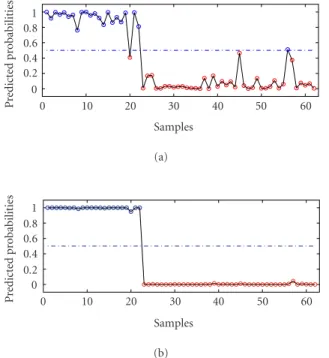
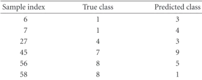
method. The average error with linear PC logistic regres-sion is 2 and the error with KPC classification is 0. The detailed results are given inFigure 2.
Lung cancer
The lung cancer dataset has 918 genes, 73 samples, and 7 classes. The number of samples per class for this dataset is small (less than 10) and unevenly distributed with 7 classes, which makes the classification task more challenging. A third-order polynomial kernelK(xi,xj)= (xixj+ 1)3, and an RBF kernel withσ=1 were used in the experiments. We chose the 100 most informative genes and 20 eigenvectors with our gene and model selection methods. The computational results of KPC classification and other methods are shown inTable 1. The results from SVMs for lung cancer, lymphoma, and NCI shown in this paper are those from Ding and Peng [11]. Six misclassi-fications with KPC and a polynomial kernel are given in Table 2.Table 1shows that KPC with a polynomial kernel is performed better than that with an RBF kernel.
Lymphoma
The lymphoma dataset has 4026 genes, 96 samples, and 9 classes. A third-order polynomial kernelK(xi,xj)= (xixj+ 1)3and an RBF kernel withσ=1 were used in our
analysis. The 300 most informative genes and 21 eigenvec-tors corresponding to the largest eigenvalues were selected with the gene selection method and AIC criteria. A com-parison of KPC with other methods is shown inTable 3.
0 0.2 0.4 P redict ed p ro babilities 0.6 0.8 1 0 10 20 30 Samples 40 50 60 (a) 0 0.2 0.4 P redict ed p ro babilities 0.6 0.8 1 0 10 20 Samples 30 40 50 60 (b)
Figure2. Outputs with (a) linear PC regression and (b) KPC classification.
Table2. Misclassifications of lung cancer.
Sample index True class Predicted class
6 6 4 12 6 4 41 6 3 51 3 6 68 1 5 71 4 3
Table3. Comparison for lymphoma.
Methods Number of errors
KPC with a polynomial kernel 2
KPC with an RBF kernel 6
PC 5
SVMs 2
Regularized logistic regression 5
Misclassifications of lymphoma using KPC with a poly-nomial kernel are given inTable 4. There are only 2 mis-classifications of class 1 using our KPC algorithm with a polynomial kernel, as shown inTable 4. The KPC with a polynomial kernel outperformed that with an RBF kernel in this experiment.
NCI
The NCI dataset has 9703 genes, 60 samples, and 9 classes. The third-order polynomial kernel K(xi,xj) = (xixj+ 1)3and an RBF kernel withσ =1 were chosen in
Table4. Misclassifications of lymphoma.
Sample index True class Predicted class
64 1 6
96 1 3
Table5. Comparison for NCI.
Methods Number of errors
KPC with a polynomial kernel 6
KPC with a RBF kernel 7
PC 6
SVMs 12
Logistic regression 6
Table6. Misclassifications of NCI.
Sample index True class Predicted class
6 1 3 7 1 4 27 4 3 45 7 9 56 8 5 58 8 1
this experiment. The 300 most informative genes and 23 eigenvectors were selected with our simple gene selection method and AIC criteria. A comparison of computational results is summarized inTable 5 and the details of mis-classification are listed inTable 6. KPC classification has equivalent performance with other popular tools.
DISCUSSIONS
We have introduced a nonlinear method, based on kPCA, for classifying gene expression data. The algorithm involves nonlinear transformation, dimension reduction, and logistic classification. We have illustrated the eff ec-tiveness of the algorithm in real life tumor classifications. Computational results show that the procedure is able to distinguish different classes with high accuracy. Our ex-periments also show that KPC classifications with second-and third-order polynomial kernels are usually performed better than that with an RBF kernel. This phenomena may be explained from the special structure of gene expression data. Our future work will focus on providing a rigor-ous theory for the algorithm and exploring the theoretical foundation that KPC with a polynomial kernel performed better than that with other kernels.
DISCLAIMER
The opinions expressed herein are those of the authors and do not necessarily represent those of the Uniformed Services University of the Health Sciences and the Depart-ment of Defense.
ACKNOWLEDGMENTS
D. Chen was supported by the National Science Foundation Grant CCR-0311252. The authors thank Dr. Hanchuan Peng, the Lawrence Berkeley National Labora-tory for providing the NCI, lung cancer, and lymphoma data.
REFERENCES
[1] Bicciato S, Luchini A, Di Bello C. PCA disjoint mod-els for multiclass cancer analysis using gene expres-sion data.Bioinformatics. 2003;19(5):571–578. [2] Yeung KY, Ruzzo WL. Principal component analysis
for clustering gene expression data. Bioinformatics. 2001;17(9):763–774.
[3] Rosipal R, Trejo LJ. Kernel partial least squares re-gression in RKHS: theory and empirical compari-son. Tech. Rep. London: University of Paisley; March 2001.
[4] Ng A, Jordan M, Weiss Y. On spectral clustering: Analysis and an algorithm. In: Advances in Neu-ral Information Processing Systems 14,Proceedings of the 2001. Vancouver, British Columbia: MIT Press; 2001:849–856.
[5] Ideker T, Thorsson V, Siegel AF, Hood LE. Test-ing for differentially-expressed genes by maximum-likelihood analysis of microarray data. J Comput Biol. 2000;7(6):805–817.
[6] Golub TR, Slonim DK, Tamayo P, et al. Molecu-lar classification of cancer: class discovery and class prediction by gene expression monitoring. Science. 1999;286(4539):531–537.
[7] Alon U, Barkai N, Notterman DA, et al. Broad patterns of gene expression revealed by clustering analysis of tumor and normal colon tissues probed by oligonucleotide arrays. Proc Natl Acad Sci USA. 1999;96(12):6745–6750.
[8] Garber ME, Troyanskaya OG, Schluens K, et al. Di-versity of gene expression in adenocarcinoma of the lung. Proc Natl Acad Sci USA. 2001;98(24):13784– 13789.
[9] Alizadeh AA, Eisen MB, Davis RE, et al. Dis-tinct types of diffuse large B-cell lymphoma identified by gene expression profiling. Nature. 2000;403(6769):503–511.
[10] Ross DT, Scherf U, Eisen MB, et al. Systematic vari-ation in gene expression patterns in human cancer cell lines.Nat Genet. 2000;24(3):227–235.
[11] Ding C, Peng H. Minimum redundancy feature selection from microarray gene expression data. In: Proc IEEE Bioinformatics Conference (CSB ’03). Berkeley, Calif: IEEE; 2003:523–528.