Schedule risk analysis of railway projects using monte-carlo simulation

Full text

(1)COPYRIGHT AND CITATION CONSIDERATIONS FOR THIS THESIS/ DISSERTATION. o Attribution — You must give appropriate credit, provide a link to the license, and indicate if changes were made. You may do so in any reasonable manner, but not in any way that suggests the licensor endorses you or your use. o NonCommercial — You may not use the material for commercial purposes.. o ShareAlike — If you remix, transform, or build upon the material, you must distribute your contributions under the same license as the original.. How to cite this thesis Surname, Initial(s). (2012) Title of the thesis or dissertation. PhD. (Chemistry)/ M.Sc. (Physics)/ M.A. (Philosophy)/M.Com. (Finance) etc. [Unpublished]: University of Johannesburg. Retrieved from: https://ujcontent.uj.ac.za/vital/access/manager/Index?site_name=Research%20Output (Accessed: Date)..

(2) Schedule risk analysis of railway projects using monte-carlo simulation. by. Motlatso Mabeba 201507351. A Mini-Dissertation. Submitted in partial fulfillment of the requirements for the degree. MASTER IN ENGINEERING MANAGEMENT. Department of Engineering and Built Environment. UNIVERSITY OF JOHANESBURG 2018.

(3) Abstract Railways have been used throughout history for the transportation of goods. Even though the inception of rail improved civilization, due to its inefficiencies, road transport is dominating the freight and logistics industry. Company A, which has the largest market share in rail has embarked on projects in an attempt to improve rail efficiencies by moving more volumes of freight timeously. Most of the projects of Company A have failed largely due to the poor planning of the projects in the feasibility stages. Most of the planning schedules are overoptimistic and thus unreliable. The scope of this study is to investigate the way in which planning schedules of Company A are developed by undertaking a schedule risk analysis and using Monte Carlo simulation to validate the schedule. If projects of Company A can be planned better, using schedule risk analysis, projects can become more successful in terms of delivering projects on time and then execute the projects on time..

(4) Table of Contents. Abstract ........................................................................................................................................... ii Table of Contents ........................................................................................................................... iii List of Figures ................................................................................................................................. v Acknowledgements ....................................................................................................................... vii Dedication .................................................................................................................................... viii 1. 2. Introduction-Schedule Risk Analysis for Company A ............................................................ 1 1.1. History of Railway .......................................................................................................... 1. 1.2. Modern Railway –Freight Business ................................................................................ 1. 1.3. Problem statement ........................................................................................................... 6. 1.4. Scope of Study ................................................................................................................ 7. 1.5. Objectives of Study ......................................................................................................... 7. 1.6. Methodology ................................................................................................................... 8. 1.7. Organization of report ..................................................................................................... 8. Literature Review .................................................................................................................... 1 2.1. Scheduling....................................................................................................................... 1. 2.1.1. Schedule as part of the triple constraint triangle ......................................................... 2. 2.1.2. Baseline Schedule ....................................................................................................... 3. 2.1.3. Presentation of a schedules ......................................................................................... 3. 2.1.4. Critical Path Method ................................................................................................... 6. 2.1.5. PERT ......................................................................................................................... 12. 2.1.6. Schedule acceleration................................................................................................ 14. 2.2 2.2.1 2.3. Monte-Carlo Methods ................................................................................................... 16 Monte Carlo Simulation............................................................................................ 17 Schedule Risk Analysis................................................................................................. 18. 2.3.1. Preparation of Project Schedule ................................................................................ 19. 2.3.2. Sources of Schedule Risks ........................................................................................ 19. 2.3.3. Schedule Uncertainty ranges..................................................................................... 21. 2.3.4. Simulation of schedule .............................................................................................. 23. iii.

(5) 2.4 3. Methodology: Schedule Risk Analysis .................................................................................... 1 3.1. 4. ‘Design of a railway exchange yard’ Specification. ....................................................... 2. 3.1.1. Topographical Survey ................................................................................................. 2. 3.1.2. Geotechnical site work ................................................................................................ 2. 3.1.3. Perway Design ............................................................................................................ 2. 3.1.4. Architectural Design ................................................................................................... 2. 3.1.5. Mechanical Design...................................................................................................... 2. 3.1.6. Electrical Design ......................................................................................................... 3. 3.1.7. Drainage Design.......................................................................................................... 3. Results and Analysis of results ................................................................................................ 1 4.1. Questionnaire 1 (Risky project Activities) ..................................................................... 4. 4.2. Questionnaire 2 (Three point Activity Estimation) ........................................................ 6. 4.3. Questionnaire 3 (Activity Distribution) ........................................................................ 11. 4.4. Monte Carlo Simulation results .................................................................................... 18. 4.4.1 4.5 5. Chapter Summary ......................................................................................................... 24. Monte-Carlo Simulation Results .............................................................................. 19 Chapter Summary ......................................................................................................... 23. Conclusion ............................................................................................................................... 1 5.1. Overview ......................................................................................................................... 1. 5.2. Study results .................................................................................................................... 1. 5.3. Recommendations ........................................................................................................... 2. 5.4. Limitations of the study .................................................................................................. 2. 6. References................................................................................................................................ 3. 7. Appendix A.............................................................................................................................. 1. iv.

(6) List of Figures Figure 1: Rail Market Share and Tonnes /km (Logistic Barometer, 2015) .................................... 2 Figure 2: PSA for project 3426783 ................................................................................................. 5 Figure 3: A PCN for extension of time for Project 3426783 .......................................................... 5 Figure 4: PSA 2 for project 3426783 .............................................................................................. 6 Figure 5: Sample WBS of a Wastewater Treatment Plant. (PMBOK Guide, 2017) ...................... 1 Figure 6: Project Management Triple-Constraint Triangle ............................................................ 2 Figure 7: Bar (Gantt) Chart (Total Quality-Key terms and concepts, 1995) .................................. 4 Figure 8: Milestone Chart. (PMBOK Guide, 2017) ....................................................................... 5 Figure 9: PDM network diagram (PMBOK Guide, 2017) ............................................................. 6 Figure 10: Flow chart showing high level development of AON diagram..................................... 8 Figure 11: Activity Identity Box ..................................................................................................... 9 Figure 12: Network Logic diagram using ADM. (PMBOK Guide, 2017) ................................... 12 Figure 13: PERT activity duration estimation (PMBOK Guide, 2017)........................................ 13 Figure 14: Comparison of schedule acceleration techniques (PMBOK,2017) ............................. 15 Figure 15: Overview of Monte-Carlo simulation technique. (Project Management in the Oil and Gas Industry, 2016) ............................................................................................................... 17 Figure 16: Monte-Carlo Process for schedule risk (GAO Cost Estimating and Assessment Guide, 2010) ..................................................................................................................................... 18 Figure 17: Triangular Distribution ................................................................................................ 22 Figure 18: Uniform Distribution ................................................................................................... 22 Figure 19: Normal Distribution .................................................................................................... 22 Figure 20: Beta Distribution ......................................................................................................... 22 Figure 21: An example of a probability distribution for the duration of an activity .................... 24 Figure 22: 'Design for Railway Exchange Yard' activities ............................................................. 1 Figure 23: Questionnaire 1: Risky project activities....................................................................... 4 Figure 24: Questionnaire 2: Results of Question 1 ......................................................................... 6 Figure 25: Questionnaire 2: Results of Question 2 ......................................................................... 7 Figure 26: Questionnaire 2: Results of Question 3 ......................................................................... 7. v.

(7) Figure 27: Questionnaire 2: Results of Question 4 ......................................................................... 8 Figure 28: Questionnaire 2: Results of Question 5 ......................................................................... 8 Figure 29: Questionnaire 2: Results of Question 6 ......................................................................... 9 Figure 30 Questionnaire 2: Results of Question 8 .......................................................................... 9 Figure 31: Questionnaire 3: Results of Question 1 ....................................................................... 13 Figure 32: Questionnaire 3: Results of Question 2 ....................................................................... 14 Figure 33: Questionnaire 3: Results of Question 3 ....................................................................... 14 Figure 34: Questionnaire 3: Results of Question 4 ....................................................................... 15 Figure 35: Questionnaire 3: Results of Question 5 ....................................................................... 15 Figure 36: Questionnaire 3: Results of Question 6 ....................................................................... 16 Figure 37: Questionnaire 3: Results of Question 7 ....................................................................... 16 Figure 38: Questionnaire 3: Results of Question 8 ....................................................................... 17 Figure 39: Screenshot of Simulation results in Primavera Risk Analysis Software: Possible completion date ..................................................................................................................... 19 Figure 40: Screenshot of Simulation results in Primavera Risk Analysis Software: Duration Estimate................................................................................................................................. 20 Figure 41: Probability Distribution ............................................................................................... 21 Figure 42: Schedule Sensitivity Index: Entire Plan ...................................................................... 22. vi.

(8) Acknowledgements I would like to acknowledge my Supervisor for his assistance, guidance and support.. vii.

(9) Dedication I dedicate this study to the following: . Malebo Mabeba. . Samuel Mabeba. . Sinah Mabeba. . Kutlwano Mabeba. . Moagi Seete. viii.

(10) 1 Introduction-Schedule Risk Analysis for Company A. 1.1 History of Railway The development of railway is one of great significance in the progression of civilization and in the development of the transportation industry at large. Transportation of goods from place to place has significantly improved with the inception of railway. Carts drawn by animals were one of the first modes of transport used but later the animals were replaced by mechanical power and in 1769, Nicholes Carnot introduced steam power to railways. Steam powered locomotives were further developed and on the 27th September 1825, a railway line between Stockton and Darlington was opened for public use. [1]. 1.2 Modern Railway –Freight Business Modern railways include electrically powered locomotives as well as locomotives that are powered by diesel. The use of railways for transportation of goods has grown steadily over time but road transport has had a substantially faster growth rate and has a larger market share in the transportation and logistics industry. The market share for railway in freight business is only between 15-25%, which is low compared to the capital cost of its infrastructure. Figure 1 provides the rail market share for different functions. The freight logistics business is a very competitive industry and even though railways are more reliable, safer, more fuel efficient, can transport greater volumes at a time, road transport still transports the highest volumes overall.. 1.

(11) In 2013, it was documented that for General Freight Business (GFB), road transport accounted for 221 billion tonne-kilometers of freight delivery while rail accounted for only 39 million tonne-kilometers (Figure 1). [2]. Figure 1: Rail Market Share and Tonnes /km (Logistic Barometer, 2015) The decline in the overall delivery of transport as well logistic services of railway in Southern Africa started in 1992 after infrastructure investment shortages and maintenance budget cuts.. 2.

(12) The Turnaround times to transport volumes of freight on rail have become significantly higher than road transportation which makes railway less efficient in terms of delivery of freight.. A company (Company A) in Southern Africa which has the largest market share in the railway industry was used in this study to investigate freight business. Due to the declining growth of railway in freight business, Company A has been embarking on major projects in the past 5 years with the objective of transferring volumes from road to rail. The introduction of these projects by Company A was greatly influenced by the need to improve efficiency of rail transport. Even though the cost of moving freight with rail is significantly cheaper, most customers still opt for road transport. [3] The type of projects that have been implemented by Company A include the following: . Upgrading of track infrastructure in order to run faster trains. . Purchasing of trains that require less maintenance. . Construction of new railway lines in order to run more routes. . Running of longer trains to transport higher volumes. With the implementation of all these projects, the expertise of experienced Project Managers was warranted to execute these projects within budget, on time and within the required quality but these projects have been poorly executed from a time management perspective leading to huge revenue losses. [4]. 3.

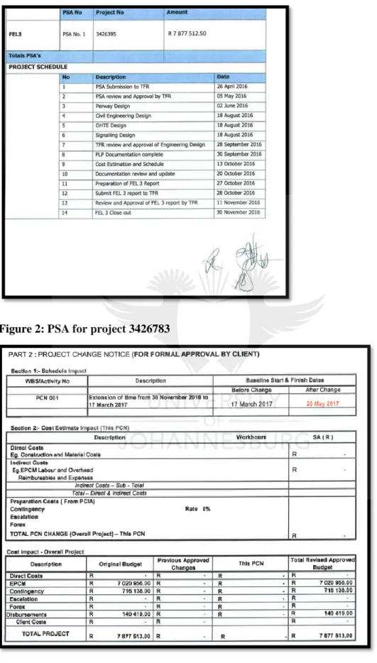
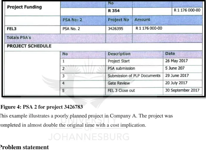
(13) It was discovered that the formative planning stages of these projects have been thoroughly neglected and overrunning of project schedules has become the norm. Late project delivery occurs with most of the projects and no time contingency has been allowed for. Most of the projects exceed the budget substantially because they are not completed within the specified durations. The schedules for the projects are unrealistic and thus projects are not able to realize benefits on the planned dates because construction is delayed. In order for projects in Company A to be completed on time, the planning of projects needs to improved, most especially the way in which the project schedules are developed.. Example of a poorly planned project in Company A A recent project in Company A undergoing feasibility study also succumbed to failure due to poor planning. The project, with project number 3426395 had an initial budget of R7 877 512.50 with the project commencing on 26 April 2016 and ending on 30 November 2016. Figure 2, shows the original Project Specific Agreement (PSA) between Company A and their client. The PSA was for a Feasibility study. The PSA gives the project budget as well as the high-level milestones for the project. . The project was given an original duration of approximately 7 months for the completion of the study.. The project, however, could not be completed within the agreed duration and thus a Project Change Notice (PCN) was sent to the client for approval for extension of time (Figure 3). As can be seen from Figure 3, the project was subsequently extended from 30 November 2016 to 17 March 2017 (An additional 3 months). No cost impact was recorded at this time.. 4.

(14) Figure 2: PSA for project 3426783. Figure 3: A PCN for extension of time for Project 3426783. 5.

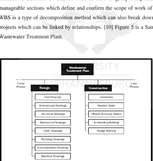
(15) Eventually, Company A had to procure external resources to fast track the project. PSA 2 had to be signed with a request for additional funds. An additional R1 176 000-00 was requested from the client and the completion date was once again rescheduled. Figure 4 shows PSA 2 for project 3426783.. Figure 4: PSA 2 for project 3426783 This example illustrates a poorly planned project in Company A. The project was completed in almost double the original time with a cost implication.. 1.3 Problem statement Project schedules for planning of projects for Company A have been seen to be overoptimistic and unrealistic and have led to late delivery of infrastructure as well as substantial revenue losses due to late execution and construction. Not enough due diligence is given to the development of these planning project schedules. The planning schedules do not incorporate risk and uncertainty which leads to project failures as most deadlines are not met.. 6.

(16) Planning schedules are developed by one planner in isolation and not enough input is provided in the development of the schedules by the project team as well other subject matter experts. With the railway industry losing freight business to road transport at a high rate, it is imperative that projects be managed better so that the required railway infrastructure is constructed within the planned time in order for the infrastructure to start generating income.This will allow for traffic volumes to be increased and efficiency to be improved.. 1.4 Scope of Study The focus of this report is to analyze a planning schedule which was developed by Company A in 2015 and to use Monte-Carlo Simulation to validate the activity durations and completion dates estimated by the planner. The planning schedule used in this study is titled ‘Design of a railway exchange yard’ and the Critical Path Method was used to develop this schedule. A railway exchange yard acts as a hub within a railway network for traction change from electrical locomotives to diesel locomotives and vice versa. A railway exchange yard may also be used for light maintenance of trains. [5]. 1.5 Objectives of Study The objectives of the report and study are as follows: . To determine whether activity durations of an existing planning schedule (Design of a railway exchange yard).for Company A were estimated accurately.. 7.

(17) . To determine whether the completion date of the existing planning schedule (Design of a railway exchange yard) for Company A is accurate and realistic.. . To validate the planning schedule (Design of a railway exchange yard) by providing a level of confidence of the completion date.. 1.6 Methodology A Schedule Risk Analysis will be done on the existing planning schedule (Design of a railway exchange yard.) for Company A. Schedule Risk Analysis is a scheduling technique used to determine activity durations by incorporating risk and uncertainty and determining whether the completion date is accurate with a certain level of confidence. [6]. Monte-Carlo simulation is then run on the schedule and the output is a probability distribution which provides a realistic completion date for the project.. 1.7 Organization of report . Chapter 1 contains following: History of railway, Modern Railway: Freight Business, Problem Statement, Scope of Study ,Objectives of Study, Methodology. . Chapter 2 is the literature review. The literature review focuses on the following topics: Scheduling, Monte-Carlo Methods, Schedule Risk Analysis. . Chapter 3 contains the detailed specification of the design of the yard as well as the methodology followed in conducting the Schedule Risk Analysis.. . Chapter 4 contains the results as well as the analysis of the results. . Chapter 5 contains the conclusions of the report. 8.

(18) 2 Literature Review 2.1 Scheduling A schedule or project plan is a major tool used in project management to monitor, manage and control project activities. A successful project must be completed on time [7]. A schedule breaks down the work that needs to be performed, within the project, into activities with durations in order to calculate the total duration required to deliver or complete the project. A project schedule is used to monitor the progress of projects when updated regularly. A project schedule can be resource and cost loaded which provides a cash-flow forecast for the project [8]. Project schedules are commonly based on a Work Breakdown Structure (WBS). A WBS is used to group components of a project into manageable sections which define and confirm the scope of work of the project A. [9] A WBS is a type of decomposition method which can also break down work into separate projects which can be linked by relationships. [10] Figure 5 is a Sample of a WBS for a Wastewater Treatment Plant.. Figure 5: Sample WBS of a Wastewater Treatment Plant. (PMBOK Guide, 2017). 1.

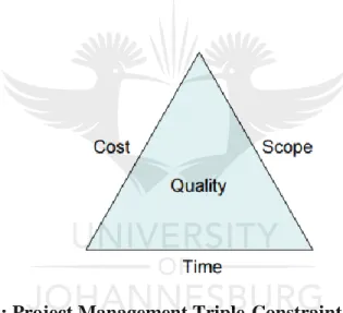
(19) 2.1.1 Schedule as part of the triple constraint triangle One of the critical project management concepts used as a framework for managing project as a whole is the project management triple constraint triangle. The three constraints, each representing a corner of the triangle are project scope, cost and time. Project scope refers to the project requirements used in order to complete project successfully. Project cost refers to the budget as well as the resources which are required to complete the project successfully. Project time refers to the schedule and duration which is required to complete the project successfully. Quality forms an integral part of each of the three constraints and is placed inside the constraint triangle. Figure 6 depicts the project management triple constraint triangle with cost, scope and time shown at each of the corners and quality inside the triangle. [11]. Figure 6: Project Management Triple-Constraint Triangle. The constraints are linked to one another as they determine the performance of a project. An extension or restriction of one of the constraints, may impact the performance of the other constraints. If for example, the scope of a project is increased, in most instances the duration and budget of the project may also increase. [12].. 2.

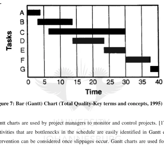
(20) 2.1.2 Baseline Schedule The baseline schedule is also known as the as-planned schedule represents the original understanding of the scope of work. The baseline schedule becomes the benchmark that the progress of a project is measured by. [13] Performance of the project can be tracked by comparing the actuals with the baseline schedule. [14]. The baseline schedule is signed off and approved by all relevant stakeholders. [9]. 2.1.3 Presentation of a schedules Schedules can be represented in many ways based on the following: . The simplicity or the complexity of project. . Detail level. . Visibility of information-graphical etc.. . Record keeping purposes. Schedules are presented in different ways depending on the purpose as well as the audience and the message that the schedule is trying to convey. [14]. Typical Schedules that are predominantly used include the following: . Gantt Charts. . Milestone Charts. . Network diagrams. 2.1.3.1 Bar (Gantt) chart Bar chart also known as Gantt charts are a graphical representation of a schedule or project plan. [9]. Gantt Charts were developed by Henry L. Gantt, an Industrial Engineer, together with Frederick W. Taylor and are still one of the most popular management tools used today. [15] Gantt Charts originated in the early 1900’s and were predominantly used for comparison of scheduled and actual progress and have continued to evolve since then. The. 3.

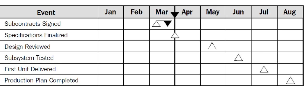
(21) initial application of Gantt charts was for production planning. [16]. The Gantt chart is widely used in project management because of its simplicity as well as its adaptability. Gantt charts (Figure 7) show the different activities in the project as a block of time, with their respective start and end dates as well as their expected durations. [9].. Figure 7: Bar (Gantt) Chart (Total Quality-Key terms and concepts, 1995). Gantt charts are used by project managers to monitor and control projects. [17] Critical Activities that are bottlenecks in the schedule are easily identified in Gantt charts and intervention can be considered once slippages occur. Gantt charts are used for progress tracking because they provide a concise outlook on the status of the project. [18]. 2.1.3.2 Milestone Charts Milestone Charts (Figure 8) are goal orientated charts similar to bar charts but only major milestone activities are shown on the vertical axis with the horizontal axis showing the start and end dates of activities. [9]. Milestone Charts are used by Project Managers for visually reporting the progress of the project at a high-level. [19] Milestone charts show case important deadlines in a project. [20]. 4.

(22) Figure 8: Milestone Chart. (PMBOK Guide, 2017). Milestones are defined as key activities in the schedule that are directly linked to achieving project objectives. Milestones include key project deliverables as well as crucial interfaces. Milestone charts do not show dependencies of activities, float or paths and are not used for giving any other information apart from providing project status. [21]. 2.1.3.3 Network Techniques (CPM and PERT). Critical Path Method (CPM) and Programme Evaluation and Review Technique (PERT) are two types of network techniques used in project scheduling. The pillar of the CPM and PERT is the network diagram. Project Network Diagrams are graphical representations of a schedule showing interdependencies and sequencing of activities within a project. [22] A network diagram is an arrangement of activities or events (milestones) which are logically tied by arcs or nodes which enable project managers to organize and also manage the project. [23]. CPM and PERT are widely used with planning and controlling of different types of projects, both small, and large. [24] CPM and PERT will be further discussed in the headings below.. 5.

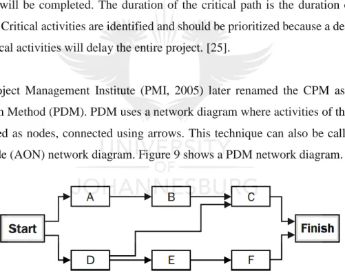
(23) 2.1.4 Critical Path Method CPM was developed in the 1950’s by Du Pont and was initially used in missile defense construction projects. CPM is widely used in Project Management for controlling cost and time of projects and uses a deterministic approach in the estimation of activity durations of a project. [8] CPM assumes a constant duration for each activities and calculates a single early start, late start as well as finish date for each activity. [9] In CPM, the total duration of the project is determined by the duration of activities in the critical path.. The CPM is defined because its main feature is the critical path. The critical path can be defined as the longest logical sequence of activities that connect the start of the project to the end of the project. The critical path can also be defined as the shortest duration that the project will be completed. The duration of the critical path is the duration of the entire project. Critical activities are identified and should be prioritized because a delay in any of the critical activities will delay the entire project. [25].. The Project Management Institute (PMI, 2005) later renamed the CPM as Precedence Diagram Method (PDM). PDM uses a network diagram where activities of the project are displayed as nodes, connected using arrows. This technique can also be called ActivityOn-Node (AON) network diagram. Figure 9 shows a PDM network diagram.. Figure 9: PDM network diagram (PMBOK Guide, 2017). 2.1.4.1 CPM: Schedule Development Development of a schedule using CPM will yield a quality product if a clear scope is defined. It is crucial that the level of detail of the schedule be defined. The level of detail is determined by the size and the complexity of the project. Once the level of detail has. 6.

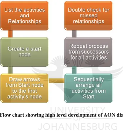
(24) been determined and set, then the project team can brainstorm and identify the activities making up the schedule. Activity identification can be done using the WBS which is the most systematic and integrated way of identifying activities in a schedule. The level of detail can be re-checked once activities have been identified to ensure that the required level is achieved.. Once activities have been identified and the level of detail has been achieved, dependencies between activities are determined and activities are sequenced.. Dependencies can either be mandatory or they can be discretionary. Mandatory dependencies are ‘hard’ dependencies and are require to be carried out at a particular time and the project mandates such a sequence. Discretional dependencies are ‘soft’ dependencies and are defined by the project team and may be defined as preferred logic. [9] Precedence relationships are then defined between the activities. CPM uses four different types of precedence relationships. The relationships are as follows: . Finish to Start : Predecessor activity must be completed before successor activity commences. . Start to Start : predecessor activity must start before successor activity may start. . Finish to Finish: Predecessor activity must be completed before successor activity must be completed.. . Start to Finish: Predecessor activity must start before successor activity is completed. [26]. Once all the precedence relationships have been identified, activity durations are determined. Duration is the estimated time required to complete the activities, usually measured in days. In CPM durations are deterministic and a single duration estimate for each activity is assigned. Once durations are determined, a network diagram can be drawn. A Start Node is drawn first either using a circle or rectangle. All activities with no predecessors will be connected. 7.

(25) to the start node. The Start Node is connected to the next activity/node using an arrow. The direction of the arrow head depicts the direction of the precedence. Activities are arranged sequentially with the last node marked as the End /Finish Node. All activities that have no successors will be connected to the End/Finish Node. Figure 10 is a flow chart showing a high level development of AON diagram.. Figure 10: Flow chart showing high level development of AON diagram. 2.1.4.2 Determining the Critical Path. Once AON network diagram has been developed, then the forward pass and backward pass method can be used. The forward pass method establishes the earliest time in which activities may be completed, while the backward pass method gives the latest time in which an activity can commence without affecting the completion date. [24] The forward pass. 8.

(26) The forward pass method starts at the start node, which is assigned a zero duration. Each of the activities in the diagram are assigned Early Start (ES) durations. ES of any activity, is the latest of the predecessor’s possible earliest finishes. [27]. ES as well as Early finishes (EF) are recorded for each node. An EF can be defined as the ES plus the duration required to complete that activity. This process is repeated for the entire network until the finish node. Backward pass The backward pass method starts at the finish node, which is assigned a zero duration. The latest possible completion is set to the earliest completion date. The Late Start (LS) and Late Finish (LF) are recorded for each of the nodes. LS of an activity can be defined as LF minus the duration of that activity. [27] The process is repeated for the entire network until the start node. Figure 11 shows is an Activity Identity box which illustrates all the possible commencements and completions of each activity within the network. [28]. . Figure 11: Activity Identity Box. 9.

(27) Critical path The critical path is then determined by the longest duration in the network. More than one (1) critical path may be identified. Slack or float can be calculated for the different activities within the network. Slack or float is can be defined by the equation below: 𝐹𝑙𝑜𝑎𝑡 = 𝐿𝑆 − 𝐸𝑆 𝑜𝑟 𝐿 Equation 1: Calculation of Float/Slack Free float is defined as the maximum duration that the activity may be delayed by without delaying the commencement of its successors. Activities in the critical path will have zero float. [29]. 2.1.4.3 Benefits of CPM The CPM is widely used in Project Management as a planning tool used to manage and control time in a project. The benefits of the CMP include: . Identification of key project activities that must be completed in a project, thus giving insight as to how the project will be executed. . The CPM identifies activities or paths that can be executed in parallel. . If resource loaded, performance and productivity can be monitored and managed. . The identification of the critical path in the project is one of the key benefits of the CPM. The critical path of the project as it provides the duration that it will take for the project to be completed and identifies activities which will have an impact on the planned completion date of the project should they be delayed. (Identifies critical activities).. . It is useful in identifying works that should be prioritized.. . It is easy to work with and through constant updating, is useful for managing progress and identifying sources of schedule risk [30]. . The CPM diagram provides a graphical representation of a schedule which allow a project manager to visually see the sequence of activities and also easily identify the critical path and activities that might slip into the critical path. [31]. 10.

(28) 2.1.4.4 Shortcomings of CPM The CPM has some shortcomings related to its application namely: . The assumption made in CPM is that the activity durations are discrete which is very unrealistic and may not yield an accurate schedule. . When using the CPM, most of the attention is focused on activities on the critical path. Some of the activities which are not on the critical path may prove to be a greater risk to the schedule, should they be delayed. [32]. . CPM may prove to be ineffective if the project is complex and there are too many activities as well as dependency relationships. The CPM diagram might become too cumbersome to comprehend and make sense of therefore it becomes difficult to manage.. . CPM cannot be used as a decision tool. [33]. 11.

(29) 2.1.5 PERT PERT was developed in 1958 by the U.S.Navy together with Booz-Allen Hamilton and the Lockheed Corporation. PERT was developed for the Polaris missile project. PERT has been widely used in Research and Development Projects. Unlike CPM , PERT does not use a deterministic activity duration estimate but uses a probabilistic activity duration estimate with the aim of determining the probability that the project will be completed in the required time frame. [34]. PMI renamed PERT as Arrow Diagram Method (ADM) in 2005. ADM is a network logic diagram where the activities in the project are shown on the arrows. It can also be referred to as Activity ON Arrow (AON) network diagram. Figure 12 is an example of an ADM network diagram. [35]. Figure 12: Network Logic diagram using ADM. (PMBOK Guide, 2017). 2.1.5.1 PERT Schedule Development Development of PERT schedule is identical to that of the CPM except for the way in which the activity durations are estimated. PERT uses the Beta distribution to estimate activity durations. [25]. In PERT network, three (3) estimates are used to model activity durations. These estimates are: . Optimistic time (a): The minimum time required for an activity to be completed.. . Realistic/ Most likely time (m): The most likely time required for an activity to be completed.. 12.

(30) . Pessimistic time (b): The maximum time required for an activity to be completed.. The weighted average duration which is the Expected Time (TE) for individual activities can be calculated with formula as given in Equation 1 with the variance given in Equation 2. The variance, also known as the standard deviation measures the uncertainty in the estimate. [25].. 𝑇𝐸 =. 𝑎 + 4𝑚 + 𝑏 6. Equation 2: Expected Time. (𝑏 − 𝑎) 2 𝜎 =( ) 𝑏 2. Equation 3: Variance for PERT method. Figure 13: PERT activity duration estimation (PMBOK Guide, 2017). 13.

(31) 2.1.6 Schedule acceleration Projects don’t always go according to plan and sometimes require external intervention in order to meet imposed deadlines or certain project objectives. Two techniques that are used in projects to accelerate or compress the schedule without a reduction in project scope are fast tracking and crashing.. Fast tracking Fast tracking schedule compression technique involves the running of activities which would otherwise be sequential in parallel for a portion of their duration. Fast tracking has an added risk of rework. [9] A disadvantage of fast tracking is that some resources might become over allocated in an effort to manage parallel activities.. Crashing Crashing is a schedule compression technique in which resources are added to the project in order to avoid overruns [36]. This technique leads to an increase in cost and some of the ways in which scheduled can be crashed include, approval of overtime, addition of human resources, paying for quicker delivery , using more expensive equipment with higher production rates. In crashing, attention is placed on activities in the critical path. [9]. Figure14 compares the two schedule compression techniques. 14.

(32) Figure 14: Comparison of schedule acceleration techniques (PMBOK,2017). 15.

(33) 2.2 Monte-Carlo Methods Monte-Carlo Methods also known as Monte-Carlo experiments are a form of computational algorithms that use repeated random sampling in order get a numerical result. Monte –Carlo Methods are used to provide approximate solutions in a number of complex physical as well as mathematical problems and have formally been used since the 1940’s. Monte-Carlo methods are collectively named after the capital city of Monaco Monte-Carlo because of the many casinos there of which the roulette wheel is one example of a random number generator. Four problems that are identified where Monte-Carlo Methods are used are: . Numerical Integration. . Simulations. . Optimization. . Generation of draws from probability distribution [37].. 16.

(34) 2.2.1 Monte Carlo Simulation Monte Carlo Simulation, also known as probability simulation is a mathematical technique which is used to model risk and uncertainty in a quantitative analysis. Monte Carlo simulation is used widely in project management, statistics, finance, insurance, research and development and in engineering. Simulations were first started in the 1930’s by Enrico Fermi and have since gained popularity in modeling different physical and conceptual systems. [25]. In Monte Carlo simulation random variables also referred to as inputs are modelled using different types of distributions and described by their statistical parameters such as mean as well as standard deviation. Distributions such as normal, log, beta, triangular, uniform etc. are used to model the input variables. Simulations are run using various programs and outputs are generated. Figure 15 provides an overview of the Monte-Carlo simulation technique.. Figure 15: Overview of Monte-Carlo simulation technique. (Project Management in the Oil and Gas Industry, 2016). 17.

(35) 2.3 Schedule Risk Analysis Uncertainty is a very big part of projects and project schedules are no exception. Risks in project schedules reduces the probability that a project will be completed within the specified duration. In order for projects to be completed on time, uncertainty needs to be considered during schedule development. Monte-Carlo Simulations are a very effective tool in determining the impact of the identified risks on the project duration and thus form a critical part in schedule risk analysis. [31] Projects sometimes experience technical challenges and schedule risk analysis addresses the probability that the planned completion date will be met with a certain level of confidence and determines the effect of activities slipping onto the schedules critical path. [38]. These are steps followed in order to perform schedule risk analysis. . Preparation of Project Schedule. . Identification of Schedule risk sources. . Estimation of 3 point activity duration ranges-assignment of probabilities. . Monte-Carlo simulation (See Figure 16 for the process). Figure 16: Monte-Carlo Process for schedule risk (GAO Cost Estimating and Assessment Guide, 2010). 18.

(36) 2.3.1 Preparation of Project Schedule In order to perform a schedule risk analysis, a schedule is prepared using the CPM. The level of detail of the schedule should be evaluated. Summary activities should be avoided as this will yield overoptimistic results. Too much information makes the process burdensome and also requires a lot more process time for the simulation. Parallel paths that converge at a single merge point should be taken note of due to the added risk and increased probability of delay at that point. This scenario is known as the mergebias which is defined as the requirement of two or more inputs before the commencement of an event. [39]. 2.3.2 Sources of Schedule Risks A schedule risk is a risk that affects the completion date of the project as scheduled. Schedule risks can lead to cost risks and performance risks. It is important that schedule risks are identified once schedule has been developed in order to mitigate the effects of the risks. The Project Experience Risk Information library (PERIL) database shows that schedule risks represent a third of the records of all types of risks and the three categories of schedule risks identified include delays, estimates as well as dependencies.. 2.3.2.1 Delays These types of risks are the most common and account for roughly half of all the schedule risks and are defined by a slippage in the project schedule if a part, a decision or if information is late. A part imperative to completing a project deliverable was noted as accounting for the most frequently reported delays. Information that is late is said to be the delay that has the greatest consequence. Also, misunderstandings and communication time lags due to outstanding or late information are common types of schedule delays. Decisions that are not made timeously by relevant stakeholders can cause schedule slippage and cause delays. [40]. 19.

(37) 2.3.2.2 Estimates Estimate schedule risks include cases where inadequate durations are allocated to activities in the schedule. This category of schedule risk is the most visible and has the greatest consequence with the subcategories including learning curves, judgment as well imposed deadlines. Good duration estimate depends heavily on historical data. Learning curves problems attribute to the highest number of estimating schedule risks and also have high impacts on the schedules. This type of estimating risk has mainly to do with the quality of the activity duration estimate with the implementation of new technology or new people in the project team. Judgment refers to over optimism when it comes to activity duration estimation. Doing a worst-case analysis is beneficial in combating over optimism as it allows for duration estimates to be more realistic. Imposed deadlines are due to deadlines that are set in advance with no input from the project team which result in unrealistic activity duration estimates and slippage in the overall schedule. [40]. 2.3.2.3 Dependencies This category of schedule risks include activities outside the project that have the potential to cause schedule slippage with the subcategories including other projects, infrastructure as well as legal issues. Other projects often with shared dependencies are the most common types of dependency schedule risks. Larger programs often have smaller projects linked by interdependencies. Slippage of the overall program becomes eminent if the required deliverables is delayed and it has an interdependency. Interface management techniques are vital for creating visibility of all interdependencies in programs in order to mitigate risks of delay. Infrastructure schedule risks are those caused by failures in systems, lack of resources, network problems as well as downtime due to maintenance. Legal issue are the schedule risks with the highest consequence when it comes to dependency schedule risks because they can potentially stop a project. It is imperative to keep abreast with changing law, regulations and standards. [40]. 20.

(38) 2.3.3 Schedule Uncertainty ranges Uncertainty is a reality when it comes to developing a project schedule and in an effort to mitigate risk and to improve the process, probabilistic /stochastic activity duration estimation is used in schedule risk analysis. [41]. Once risks have been identified and mapped to the suitable activities, a three (3) point activity duration estimate is assigned to each activity. [42] Just like the PERT method, an optimistic, pessimistic and most-likely duration estimate is allotted to each activity. Unlike PERT method which uses the Beta distribution to model activity durations, schedule risk analysis uses a range of distributions to accurately model each activity. A distribution function is determined for each activity taking into consideration the uncertainty in completing each activity. [41]. Frequently used probability distribution in schedule risk analysis are Triangular, Beta, normal, uniform. [43] . The Triangular Distribution (Figure 17) is one of the most commonly used distribution in activity duration estimation. [31]. The triangular distribution can either be symmetrical, skewed to the left or to the right and is bounded by the optimistic and the pessimistic duration. [44]. . The Uniform Distribution (Figure 18) is a constant distribution with the optimistic, pessimistic and most-likely values all equal to each other.. . The Normal Distribution (Figure 19) is a symmetrical, continuous distribution which is defined by the standard deviation, as well as the mean. [45]. Normal distribution can be described as being a bell-curve. [46]. . The Beta Distribution (Figure 20) was first developed in the 1950’s with its application mainly on modeling uncertainty in complex projects. [44]. It’s a normal distribution which has either a negative or a positive skew.. .. 21.

(39) Figure 17: Triangular Distribution. Figure 19: Normal Distribution. Figure 18: Uniform Distribution. Figure 20: Beta Distribution. 22.

(40) 2.3.4 Simulation of schedule Once the schedule has been prepared using the CPM, risks identified and activity ranges and distributions have been determined, Monte –Carlo Simulation can be run in order to determine with a certain level of confidence if the completion date is realistic. The purpose of a simulation is to replicate real life problems using a set of defined assumptions. This method makes it easy to control risk in a project schedule and is a good decision –making tool. [41]. The Monte-Carlo simulation for schedule risk analysis answers three very critical questions in project management. . Is the completion date of the project, or the duration provided to complete the project realistic?. . Is the duration provided, the most-likely duration?. . How much more time can be allocated as contingency in order to reduce the overrun risk exposure?. During the each iteration of the Monte-Carlo Simulation, a random value, bounded by the activity ranges as well as the pre-arranged distribution function is selected for each risky activity. The number of iteration selected, depends on the complexity of the schedule. Generally, the more iterations that are simulated, the more accurate the output becomes. Usually thousands of iterations are computed in a Monte-Carlo Simulation. [47] Each iteration may yield a different completion date, a different project duration and possibly a different critical path may identified. All these different outputs are stored in which ever program is used for the Monte-Carlo Simulation. Once the simulation is compete, possible completion dates which have been computed for each iteration are displayed in a graph or table showing the relative frequency of the possible completion dates. [48] Figure 21 shows an example of a probability distribution duration for one activity within a project schedule.. 23.

(41) Figure 21: An example of a probability distribution for the duration of an activity. 2.4 Chapter Summary Scheduling is a major tool used in projects to plan, monitor as well as to control the activities within a project. A project is considered successful if it is completed before or on the completion date. A schedule is a very critical component in the triple constraint triangle and failure to complete a project on time may have adverse effect on the delivery of the other constraints.. Schedules may be presented in various ways and may be tracked against the baseline schedule. CPM and PERT method are highly used in project management. Monte –Carlo simulations are used in scheduling, together with the CPM to produce an optimized project schedule. Schedule Risk analysis uses Monte-Carlo simulations to model project schedules and to account for potential risks in the project. 24.

(42) 3 Methodology: Schedule Risk Analysis In order to perform Schedule Risk Analysis ‘Design of a railway exchange yard’ schedule, the following steps were undertaken: 1. A schedule was prepared using the CPM in Primavera P6 software using the “Design of a railway exchange yard’ specification. 2. A Questionnaire (Questionnaire 1) was conducted using SurveyMonkey to identify the 10 keys activities in the schedule with the highest risk. 3. Two Questionnaires were then prepared using SurveyMonkey distributed togetjer with the ‘Design of a railway exchange yard’ specification. a. Questionnaire 2 was titled: Three point Estimation. The purpose of this questionnaire was to use the three point duration estimation technique to estimate activity durations of the 10 activities identified as having the highest risk. b. Questionnaire 3 was titled: Activity distribution. The purpose of this questionnaire was to identify the distribution function for each of the 10 risky activities in the schedule. 4. Once the three point duration estimation and distribution have been identified, the information is inputted in Primavera P6 software (Risk Analysis Software) and a MonteCarlo simulation is run. 5. The output from the Monte-Carlo Simulation include the following: a.. Probability distribution, with the expected completion date. b. Tornado chart with provides sensitivity of the results.. 1.

(43) 3.1 ‘Design of a railway exchange yard’ Specification. 3.1.1 Topographical Survey 1. Topographical Survey of 500 Ha. 3.1.2 Geotechnical site work 1. 38 Tractor Loaded Backhoe (TLB) test pits to profile soils, investigate soil strengths/capacities and identify potential problem soils on site; 2. 38 Dynamic Probing Super Heavy (DPSH) Tests, and; 3. 9 percussion boreholes;. 3.1.3 Perway Design 1. Track Design of railway yard of 4 arrival/departure lines 2. 16 km of railway track overall 3. Geometric design of railway track 4. Earthwork design of railway track. 3.1.4 Architectural Design 1. Design of the flowing buildings: o Administration building north (75m2 ) o Administration building south (75m2 ) o Staff amenities building (65m2 ) o Shunters and guard cabin facilities (30m2 ) o Locomotive provisioning facility (30m2 ). 3.1.5 Mechanical Design The mechanical design includes description of the mechanical systems in the 5 buildings. The nominated systems to be implemented are as follows: 1. Air-conditioning System 2. Ventilation system. 2.

(44) 3. Hot and Cold Water Reticulation System 4. Fire protection system. 3.1.6 Electrical Design 1. Bulk Power Supply of Yard 2. Lighting of buildings and yard 3. Over Head Track Equipment (OHTE) 4. Signaling Design. 3.1.7 Drainage Design 1. Side drains 2. Sub surface drainage 3. Culvert design 4. Storm water design 5. Sewer design. 3.

(45) 4 Results and Analysis of results The activities of ‘Design of a railway exchange yard’ schedule that was developed by the planner of Company A can be seen in Figure 22. The full schedule with the Gantt chart can be seen in the Appendix. A. The schedule starts on the 9th March 2015 and the completion date is the 11 October 2016. The CPM was used to develop the schedule with the mostlikely duration estimate used to develop the schedule. All relationships are FS (Finish to Start). Figure 22: 'Design for Railway Exchange Yard' activities. 1.

(46) The Questionnaires were distributed to the project team from Company A in order to validate ‘Design of a railway exchange yard’ schedule. The sample sizes used for each of the questionnaires can be seen in Tables 2-4. The questionnaire was distributed to the entire project team of Company A. The sample size larger than 20 independent project team is deemed sufficient in schedule development for feasibility studies as it is able to reduce potential bias. [49] The schedule used in the study is a planning for design schedule therefore the project team selected included to complete the questionnaires included: . Planners of various technical backgrounds and skills. . Project Managers. . Design Engineers for different disciplines. The selection of the project team was based on the project deliverables and the sample was representative of all the key stakeholders as well as the project team members responsible for completion of tasks in the schedule. In order for schedule development to be effective, the relevant stakeholders should be represented during the development phase of the schedule. In many projects, one planner or scheduler develops the schedule in isolation which is not deemed as best practice. It is recommended that all stakeholders performing the works in the schedule be part of the development process in order for an accurate baseline schedule to be created. [50]. 2.

(47) Table 1: Questionnaire 1 Sample size Planners Project Managers/Construction Managers. Design Engineers. Total. 10. 10. 35. 15. Table 2: Questionnaire 2 Sample size Planners Project Managers/Construction Managers. Design Engineers. Total. 10. 10. 30. Planners Project Managers/Construction Managers. Design Engineers. Total. 15. 10. 30. 10. Table 3: Questionnaire 3 Sample size. 10. 3.

(48) 4.1 Questionnaire 1 (Risky project Activities) The purpose of Questionnaire 1 (Figure 23) was to identify activities in the schedule that had the highest source of risk according to the project team. All the activities in the ‘Design of railway yard’ schedule were inputted as part of Questionnaire 1. (Figure 20), using Survey Monkey. The questionnaire was then distributed to the project team for their input. Activities with the highest risk source do not necessarily form part of the critical path. Thus, identification of risky activities in schedule risk analysis is an improvement to the critical path method. [51]. Figure 23: Questionnaire 1: Risky project activities. 4.

(49) Results of Questionnaire 1 The results of Questionnaire 1 can be seen in Table 5. The results (in percentages) show the activities identified by the project team as having the highest risk source. The percentages show the activities that the project team deemed to be the most risky activities. The activities that are highlighted in green are the ones with the highest risk as per the survey. As can be seen from the Table 5, Perway and Architectural designs are the activities were seen to have the highest risk. This might be due to the fact that these activities are the first to commence and are the main disciplines in engineering designs and if delayed, they delay the start of other engineering designs such as structural, electrical and mechanical.. Table 4: Results of Risky activities selected by project team. 5.

(50) 4.2 Questionnaire 2 (Three point Activity Estimation) The purpose of Questionnaire 2 was to determine the activity durations of the identified risky activities using the three point estimation method. Probabilistic duration estimation is a good technique to use when there is great deal of uncertainty in activity durations. [52]. The optimistic, most-likely and pessimistic durations for each activity was provided and the average duration (in weeks) for each activity was calculated. Figure (24-30) show the questions asked in the questionnaire, with a graph and table providing the average durations (in weeks) that were estimated by the project team for the optimistic, most-likely and pessimist activity durations.. Figure 24: Questionnaire 2: Results of Question 1. 6.

(51) Figure 25: Questionnaire 2: Results of Question 2. Figure 26: Questionnaire 2: Results of Question 3. 7.


(53) Figure 29: Questionnaire 2: Results of Question 6. Figure 30 Questionnaire 2: Results of Question 8. 9.

(54) Questionnaire 2 provides the probabilistic duration estimation for the activities deemed as risky by the project team. . The three point estimation method models the activity durations of each the activities. This provides a better estimate for activity duration estimates as it accounts for all the possible durations for activity completion while accounting for the inherent risks.. 10.

(55) 4.3 Questionnaire 3 (Activity Distribution) The purpose of Questionnaire 3 was to determine the distribution that best modeled the activity. In order for the project team to select the appropriate distribution the typical application of each of the distributions had to be provided according to literature. The typical four distributions used in schedule development (Krige, 2016) and used as part of Questionnaire 3 include the following: . Normal. . Beta-pert. . Triangular. . Uniform. These distributions are deemed satisfactory when derived from interviews or surveys. [38]. A study was done in which the significance of input distributions was tested. The study was entitled: Suitability of different probability distributions for performing schedule risk simulations in project management. The study analyzed the use of different distributions for modelling activity durations to see if they greatly affected the completion date of the project. The results showed that the input distributions did not greatly affect the completion date of the project when using monte-carlo simulation but it is important to try and model the activity correctly as per best practice. [53]. 11.

(56) This study gives comfort that even though all distributions might not 100 % fit the activity, the results will not be affected greatly.. Typical applications of input distributions Normal distribution: Generally used for cost estimation. This distribution is not that useful for modelling asymmetrical risk but rather for the scaling of estimation error. This distribution is not typically used for duration estimation in scheduling because of its symmetry. Beta-Pert: Typically used when there is uncertainty or risk in the activity. May also be used when there is limited historical data. This makes this type of distribution the most preferred for schedule development. Typically used for modelling engineering data. [38] Triangular: This distribution is used to model technical uncertainty e.g. Architecture or engineering design. [38] Normal: Typically used when all possibilities are likely and also for engineering applications.. The project team selected the distributions that best represented the activities and the results are provided in graphs and tables as percentages of the total number of respondents. . (Figure 31-38). The distributions were then validated by literature to ensure that the correct distributions were provided.. 12.

(57) Figure 31: Questionnaire 3: Results of Question 1. 13.




(61) Figure 38: Questionnaire 3: Results of Question 8. 17.

(62) 4.4 Monte Carlo Simulation results In order to perform a Monte-Carlo simulation, the ‘Design for railway exchange yard’ schedule was inputted into Primavera Risk Analysis Software. As per Questionnaire 2 and Questionnaire 3, the optimistic, most likely and pessimistic durations were inputted into the software together with the preferred distribution functions. 1000 Monte-Carlo iterations were performed on the schedule. Table 6 summarizes the risky activities together with durations as well as distributions that were inputted into the software in order to perform a Monte-Carlo Simulation.. Table 5: Summary of activity durations and distributions Activities. Optimistic. MostLikely. Pessimistic. Distribution. Site Survey. 6. 9. 12 BetaPert. Geotechnical Fieldwork and report. 8. 10. 14 BetaPert. Perway Design. 4. 5. 8 Triangle. Drainage Design. 4. 5. 8 Triangle. Architectural Design. 6. 8. 10 BetaPert. Mechanical Design. 3. 6. 8 Triangle. Environmental: Water Use Licence. 52. 52. 52 Uniform. Municipal Submissions. 17. 24. 33 BetaPert. 18.

(63) 4.4.1 Monte-Carlo Simulation Results Figure 39 is a screenshot taken form the Primavera Risk Analysis Software which details the possible completion dates of the project. As can be seen from the figure, the number of iterations successfully completed is 1000. Each bar in the figure represents a week and minimum, maximum and mean durations are provided. The highlighters include the confidence level with which the expected completion date is expected.. Figure 39: Screenshot of Simulation results in Primavera Risk Analysis Software: Possible completion date. 19.

(64) Figure 40 is a screenshot taken from the Primavera Risk Analysis Software which details the duration estimation of the project. As can be seen from the figure, the number of iterations successfully completed is 1000. Each bar in the figure represents a week and minimum, maximum and mean durations are provided in weeks .The highlighters include the confidence level with which the expected completion date is expected.. Figure 40: Screenshot of Simulation results in Primavera Risk Analysis Software: Duration Estimate. 20.

(65) Figure 41: Probability Distribution Figure 41 shows the probability distribution (frequency histogram) for all the possible completion dates for the project. Figure 41 also shows the cumulative frequency curve Using the cumulative frequency curve, one is able to determine with a certain confidence level when the project will be completed. From the graph, the completion date with a 50% confidence level is 7 /10/2016. The completion date with an 80 % confidence level is 7/11/2016. The completion date with 100% completion level is 14/12/2016.. 21.

(66) The original completion date of the schedule before simulation was done was 11/10/ 2016. This shows that the original schedule was optimistic and unrealistic and did not account for risk.. Figure 42: Schedule Sensitivity Index: Entire Plan The Tornado graph in Figure 42 displays activities that have the highest risk. The tornado chart shows the activities with the highest sensitivity and thus the activities that have the greatest effect on the schedule. The tornado chart is based on metric Schedule Risk index (SSI). As can be seen from the sensitivity analysis the following activities have the highest sensitivity and overall highest influence on the schedule: . Application of Water Use License. . Geotechnical Field work and report. 22.

(67) . Procurement of Geotechnical studies.. 4.5 Chapter Summary Questionnaire 1 was used to identify activities in the schedule that were regarded as risky. By virtue of identification of risky activities the team becomes more aware of activities that they need to track and manage as the delay in those activities might have adverse effects on the schedule.. Questionnaire 2 was used to model the activity durations. By virtue of modeling the activity durations, the project team become aware of the possible end dates of each activity. This allows for contingency or mitigation measures to be put in place if the activity is not completed at the most likely estimated duration.. Questionnaire 3 allows for the preferred distribution or best fit to model the activity as accurately as possible.. Monte Carlo simulation was run on the schedule and a 1000 iterations were performed. The results show that the original date of completion was underestimated and contingency was required in order to account for possible risk materialization. The tornado graph highlighted the activities that have the highest sensitivity and that affect the schedule the most.. 23.

(68) 5 Conclusion 5.1 Overview The objective of the study was to validate the ‘Design of Railway Exchange Yard’ schedule that was developed by Company A and prepared by the planner. Company A has been planning projects for years and it became evident that most of the planning schedules are not completed on time due to overoptimistic, unrealistic schedules. As part of this study the ‘Design of Railway Exchange Yard’ schedule was analyzed and risky activities were identified as part of Schedule Risk Analysis. The schedule was inputted into Primavera Risk Analysis and activity durations and distributions inputted after information was collected using SurveyMonkey.. 5.2 Study results This study has shown the importance of risk identification in the development of project schedules. The original planning schedule ‘Design of Railway Exchange Yard’ did not account for risk and all activity durations were deterministic. The planner had developed the schedule in isolation with no input from the project team which leads to an unbiased schedule. The schedule risk analysis performed on the schedule provided guidance as to which activities had the highest risk source and which activities had the potential to delay the entire project. The schedule risk analysis provided a confidence level as to when the project would be completed, which allows the team to rely on the information.. 1.

(69) As per the results, the projected completion date based on Monte-Carlo Simulation was 14/12/2016 which is two months more than the original estimated completion date. This proves that the original schedule for ‘Design of Railway Exchange Yard ‘completed in 2015 was overoptimistic and unrealistic.. 5.3 Recommendations It is recommenced, as per the results of this study that Company A use schedule risk analysis to develop all planning schedules and also include the project team in the development phase of the project schedules. Schedule risk analysis accounts for risk and uncertainty and once mitigation measures are put in place, the schedule can be managed with ease. Company A will thus be able to plan for the execution of projects the planned dates and contraction of infrastructure can be managed.. 5.4 Limitations of the study The study could be improved by using more iterations in the monte-carlo simulation. More iterations leads more accurate results. SurveyMonkey only allows for 10 questions to be imputed into the survey. There is limited studies done on allocation of probability distributions to activities in a schedule. Thus, this study had to use expert judgment to be able to determine the best fit distribution for activity durations. Results could be improved by using consultants outside of Company A, in order to reduce biased results.. 2.

(70) 6 References. [1 S. Chandra and M. M. Agarwal, Railway Engineering (2nd Edition), Oxford: Oxford ] University Press, 2013. [2 . N. Viljoen and D. King, "Logistic Barometer," 2015. [Online]. Available: ] https://www.sun.ac.za/english/faculty/economy/logistics/Documents/Logistics%20B arometer/Logistics%20Barometer%202015%20Report.pdf. [Accessed 23 September 2017]. [3 S. Scott, "Market Analysis: The South African Transport and Logistics Industry - An ] Industry in Turmoil," Samrt Procurement, Cape Town, 2007. [4 S. Barradas, "Engineering News," 2 10 2016. [Online]. Available: ] http://www.engineeringnews.co.za/article/durban-port-upgrade-and-expansionproject-south-africa-2017-01-20/rep_id:4715/company:transnet-port-terminals. [Accessed 12 5 2017]. [5 S. Fedtke and N. Boysen, "A comparison of different container sorting systems in modern ] rail-rail transshipment yards," Transportation Research Part C: Emerging Technologies, vol. 82, pp. 63-87, 2017. [6 L. Tao, D. Wu, S. Lui and J. Lambert, "Schedule risk analysis for new-product development: ] The GERT method extended by a characteristic function," Reliability Engineering & System Safety, vol. 167, pp. 464-473, 2017. [7 A. Patel, P. A. Bosela and N. J. Delatte, "1976 Montreal Olympics: Case Study of Project ] Management Failure," Journal of Performance of Constructed Facilities, vol. 27, no. 3, 2013. [8 J. Meredith and S. Mantel Jr, Project Management, A Mangerial Approach, Danvers: John ] Wiley & Sons, Inc., 2009. [9 Project Management Institute, A Guide to the Project Management Body of Knowledge ] (PMBOK® Guide), Newtown Square: Project Management Institute, 2013. [1 X. Shi , J. Zheng and H. Wei, "Construction of Agricultural Logistics Operation Mode Based 0 on WBS," International Conference of Logistics Engineering and Management ] (ICLEM) 2010, 2010.. 3.

(71) [1 C. J. V. W. a. J. H. C. P. a. L. Pretorius, "Theory of the triple constraint — A conceptual 1 review," : Industrial Engineering and Engineering Management (IEEM), 2012 IEEE ] International Conference , 2012. [1 T. S. Mokoena, J. H. C. Pretorius and C. J. V. Wyngaard, "Triple constraint considerations in 2 the management of construction projects," Industrial Engineering and Engineering ] Management (IEEM), 2013 IEEE International Conference, 2013. [1 K. Sears, G. A. Clough, R. H. Rounds and . J. L. Segner, CoConstruction Project 3 Management - A Practical Guide to Field Construction Management (6th Edition), ] John Wiley & Sons, 2015. [1 A. Rodolfo and L. Mario, Dynamic Scheduling® with Microsoft® Project 2013 - The Book 4 by and for Professionals, J. Ross Publishing, Inc., 20165. ] [1 J. M. Wilson , "Gantt charts: A centenary appreciation," European Journal of Operational 5 Research, vol. 149, no. 2, p. 430–437, 2003. ] [1 J. M. Wilson, "Gantt charts: A centenary appreciation," European Journal of Operational 6 Research, vol. 149, no. 2, pp. 430-437, 2003. ] [1 A. W. Swan, "The gantt chart as an aid to progress control," Journal of the Institution of 7 Production Engineers, vol. 21, no. 10, pp. 402 - 414, 1942 . ] [1 R. T. D. G. L. Westcott, The Certified Quality Improvement Associate Handbook, Third 8 Edition, Wisconsin: American Society for Quality, 2015. ] [1 J. Levitt, Fundamentals of Space Systems (2nd Edition), Oxford University Press, 2005. 9 ] [2 L. Albert, Project Management, Planning and Control - Managing Engineering, Construction 0 and Manufacturing Projects to PMI, APM and BSI Standards (7th Edition), Elsevier, ] 2017. [2 V. L. Pisacane, Fundamentals of Space Systems (2nd Edition), Oxford University Press, 1 2005. ]. 4.

No results found