Autonomous obstacle avoidance and positioning control of mobile robots using fuzzy neural networks

Pontificia Universidad Católica del Perú

Escuela de Posgrado

Tesis de Maestría

Autonomous Obstacle Avoidance and Positioning

Control of Mobile Robots Using Fuzzy Neural Networks

Para obtener el grado de:

Magíster en Ingeniería de Control y Automatización

Presentado por: Anna-Maria Stephanie Grebner

Tutor Responsable (TU Ilmenau): Prof. Dr.-Ing. Johann Reger Professor Responsable (TU Ilmenau): Prof. Dr. Kai Wulff Professor Responsable (PUCP): Prof. Dr. Antonio Manuel

Moran Cárdenas

Declaration

I declare that the work is entirely my own and was produced with no assistance from third parties.

I certify that the work has not been submitted in the same or any similar form for assessment to any other examining body and all references, direct and indirect, are indicated as such and have been cited accordingly.

(Anna-Maria Grebner) Ilmenau, 17 September 2018

Abstract

Navigation and obstacle avoidance are important tasks in the research field of au- tonomous mobile robots. The challenge tackled in this work is the navigation of a 4- wheeled car-type robot to a desired parking position while avoiding obstacles on the way. The taken approach to solve this problem is based on neural fuzzy techniques. Earlier works resulted in a controller to navigate the robot in a clear environment. It is extended by considering additional parameters in the training process. The learning method used in this training is dynamic backpropagation.

For the obstacle avoidance problem an additional neuro-fuzzy controller is set up and trained. It influences the results from the navigation controller to avoid collisions with objects blocking the path. The controller is trained with dynamic backpropagation and a reinforcement learning algorithm called deep deterministic policy gradient.

Kurzfassung

Navigation und Hindernisvermeidung sind wichtige Aufgaben im Forschungsbereich autonomer mobiler Robotik. In dieser Arbeit wird die kollisionsfreie Navigation eines Roboters mit 4 Rädern in eine Zielparkposition behandelt. Der gewählte Ansatz um das Problem zu lösen basiert auf Techniken aus dem Neuro-Fuzzy Bereich.

In früheren Arbeiten entstand bereits ein Regler mit welchem der Roboter in einer hinder- nisfreien Umgebung navigiert werden konnte. Dieser wurde erweitert indem zusätzliche Parameter in den Trainingsprozess mit einbezogen wurden. Die angewandte Lernmetho- de ist Dynamic Backpropagation. Für die Hindernisvermeidung wurde ein zusätzlicher Neuro-Fuzzy-Regler eingerichtet und trainiert. Dieser beeinflusst die Ergebnisse des Navigationsregler um Kollisionen mit Objekten zu vermeiden. Für das Training des Reglers kommen Dynamic Backpropgation und ein reinforcement learning-Algorithmus,

genannt ’Deep Deterministic Policy Gradient Learning’, zum Einsatz.

Das entwickelte Navigationssystem konnte in verschiedenen simulierten Szenarien ge- testet werden. Der Roboter war in der Lage ohne Probleme beliebige Parkpositionen anzufahren und verschieden geformte Linien zu verfolgen.

Contents

3.1 Fuzzy Inference Systems ... 5

3.1.1 Fuzzy Sets and Fuzzy Logic ... 5

3.1.2 Fuzzy Inference Systems ... 7

3.2 Neural Network ... 11

3.2.1 Structure of Neural Networks... 11

3.2.2 Standard Backpropagation ... 12

3.2.3 Dynamic Backpropagation ... 14

3.2.4 Reinforcement Learning with an Actor-Critic-Algorithm ... 15

3.3 Fuzzy Neural Networks ... 18

3.4 Neuro-Fuzzy-Control in Robot Navigation ... 20

4 Implementation 22 4.1 Model ... 22

4.2 Navigation ... 23

4.2.1 Structure of the Neuro Fuzzy Controller ... 23

4.2.2 Training with Dynamic Backpropagation ... 26

4.3 Obstacle Avoidance ... 32

4.3.1 Structure of the Neuro Fuzzy Controller for Obstacle Avoidance . 32 4.3.2 Simulation of Obstacle Recognition ... 34

4.3.3 Training with Dynamic Backpropagation ... 35

Contents

Contents

5 Results 40

5.1 Results of the Navigation Controller ... 40 5.2 Results of the Obstacle Avoidance Controller ... 44

6 Conclusion 47

C

Bib

o

n

t

e

n

ts

Chapter 1

Introduction

Robots are growing more and more important in our modern world. Whether to make our life easier or take over dangerous tasks, their presence in our daily life has been increasing in the recent years. Especially autonomous mobile robots can already be found in many everyday applications. Museums and stores employ them to guide visitors and floor-cleaning or lawn-mowing robots made their way in many homes. In order to move around in the environment without problems, good navigation and obstacle avoidance systems areessential formobilerobots. They guarantee that therobotreaches desired positions in time and does not collide with structures and objects on the way. In this thesis a control system for a navigation and obstacle avoidance problem is developed, implemented and tested. The task consists of navigating an autonomous 4-wheeled cartype robot in a desired parking position, while avoiding collision with obstacles on the way. The techniques used to realize the controller belong in a category called fuzzy neural networks. They are hybrid systems consisting of elements from fuzzy inference systems and artificial neural networks. The strength of fuzzy systems lies in the possibility to create a system based on expert knowledge. Neural networks are known for their ability to learn and adapt to new situations. Neuro-fuzzy networks combine the advantages of both approaches by considering a fuzzy inference system as a neural network and apply training algorithms to improve their performace. The training methods used in this thesis are dynamic backpropagation and deterministic policy gradient.

This work is structured as follows: In chapter 2 the problem to be solved in this thesis is layed out in detail. Chapter 3 contains the theoratical foundations needed to understand this work. In chapter 4 a complete description on how the the controllers and learning algorithms were implemented is given. Chapter 5 presentes the results

1 Introduction

reached with the controllers in different test scenarios, followed by the conclusion in chapter 6.

Chapter 2

Problem Description

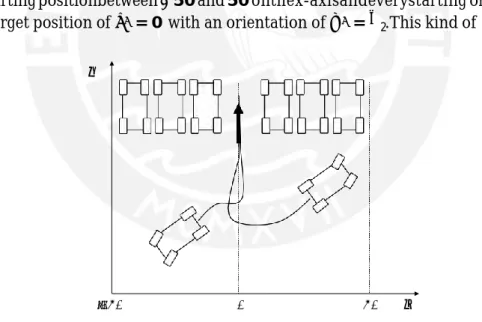
The task for this thesis is to develop a neuro fuzzy controller capable of navigating a 4-wheeled robot in the x-y-plane to a goal position. The problem is designed to be parking situation in which the robot has to move backwards in its designated spot. In the first part, the path to the goal position is clear and the robot should simply be able to reach it. This problem is shown in figure 2.1. The robot should be able to get from everystarting positionbetween −50 and 50 onthex-axisandeverystarting orientation to the target position of x∗= 0 _{with an orientation of φ}∗= π_{2. This kind of problem}

𝑦

−50 0 50 𝑥

Figure 2.1 – Parking problem to be solved

was once before tackled in [1] and a neuro-fuzzy controller was developed. Dynamic backpropagation was used in training, to adapt the parameters in the consequence part of the fuzzy controller. It lacked, however, the training of the premise parameters, which is to be added in the framework of this thesis.

2 Problem Description

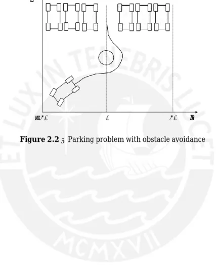
In the second part of the problem the robots way to the goal position is blocked by an obstacle, like shown in figure 2.2. The navigation controller is to be extended by the functionality to avoid obstacles. The solution should again be found by applying neuro-fuzzy techniques. A structure for the obstacle avoidance controller has to be set up and trained to fulfill the task.

𝑦

−50 0 50 𝑥

1

Chapter 3

Foundations

3.1

Fuzzy Inference Systems

3.1.1

Fuzzy Sets and Fuzzy Logic

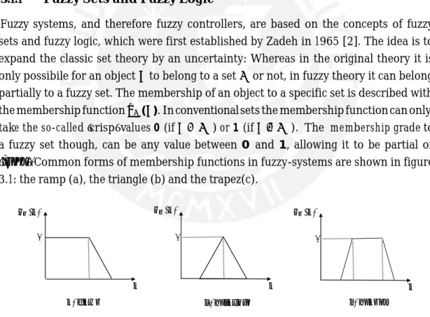
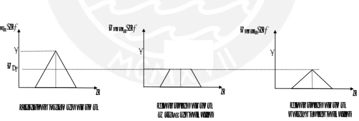
Fuzzy systems, and therefore fuzzy controllers, are based on the concepts of fuzzy sets and fuzzy logic, which were first established by Zadeh in 1965 [2]. The idea is to expand the classic set theory by an uncertainty: Whereas in the original theory it is only possibile for an object a to belong to a set M or not, in fuzzy theory it can belong partially to a fuzzy set. The membership of an object to a specific set is described with the membership function µM(a). In conventional sets the membership function can only take the so-called ’crisp’ values 0 (if a ∈M ) or 1 (if a ∈/ M ). The membership grade to a fuzzy set though, can be any value between 0 and 1, allowing it to be partial or

’fuzzy’. Common forms of membership functions in fuzzy-systems are shown in figure 3.1: the ramp (a), the triangle (b) and the trapez(c).

𝜇𝑀(𝑎) 𝜇𝑀(𝑎) 𝜇𝑀(𝑎)

1

𝑎 𝑎 𝑎

𝑎) 𝑅𝑎𝑚𝑝 𝑏) 𝑇𝑟𝑖𝑎𝑛𝑔𝑙𝑒 𝑐) 𝑇𝑟𝑎𝑝𝑒𝑧

Figure 3.1 – Common forms of fuzzy membership functions

Fuzzy sets allow to characterize states without giving a strict classification. The human language contains a lot of options to describe things in a vague way, like e.g. ’a

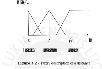
3 Foundations little bit’, ’a lot more’ or ’almost’. That is why fuzzy sets are a perfect instrument for transforming human language statements into a structure that can be treated formally exact. An example is given in figure 3.2, which shows a fuzzy description of a distance. The fuzzy variable is the distance d, which can be charaterized by the fuzzy sets ’ZERO’, ’NEAR’ and ’FAR’. A distance of 0 gets full membership in the set ’ZERO’. A distance

𝜇(𝑑)

0

5

1

0

𝑑

𝑍𝐸𝑅𝑂

𝑁𝐸𝐴𝑅

𝐹𝐴𝑅

Figure 3.2 – Fuzzy description of a distance

of 5 is considered as ’NEAR’ and every distance of 10 or greater is ’FAR’. The fuzzy sets allow to describe also distances in between. A distance of 3 for example would have

partial membership grades in the sets ’ZERO’ and ’NEAR’. It could be described as

’close to zero’, ’almost zero’ or ’very near’. As fuzzy sets in practise are often connected

with a linguistical interpretation like this, they’re also called ’linguistic variables’.

In order to work with fuzzy variables it is necessary to establish connecting opera- tors. Crisp variables can be linked with the boolean operators from standard logic. The definition of these were extended for fuzzy variables. Different applications resulted in different forms of this adaption. The most common ones are explained below.

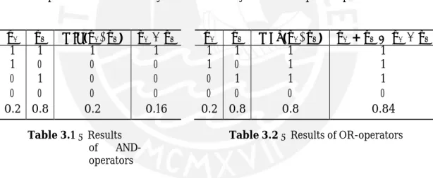
• AND operation (∧)

The first definition of a fuzzy AND-operator was proposed in [2] and uses a minimum operation

µA∧B= min(µA, µB) (3.1) As for optimization processes differentiability is often a requirement another definition can be used

3 Foundations µA µB min(µA, µB) µA · µB 1 1 1 1 1 0 0 0 0 1 0 0 0 0 0 0 0.2 0.8 0.2 0.16 µA µB max(µA, µB) µA + µB− µA · µB 1 1 1 1 1 0 1 1 0 1 1 1 0 0 0 0 0.2 0.8 0.8 0.84 • OR operation(∨)

The two most commonly used definitions for the OR-operator are the maximum operation

µA∨B= max(µA, µB) (3.3) and the algebraic sum

µA∨B= µA+ µB−µA· µB (3.4)

• NOT operation

The NOT-operation of a membership grade is determined by the difference between 1 and the degree

µ_A = 1 −µA (3.5)

The tables 3.1 and 3.2 show that these definitions are consistant with the results from boolean operators and how they work on a fuzzy membership example

Table 3.1 – Results

of AND-

operators

Table 3.2 – Results of OR-operators

3.1.2

Fuzzy Inference Systems

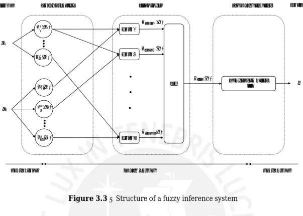
Fuzzy inference systems (FIS) are systems which describe functions by mapping inputs to outputs with the help of fuzzy sets and fuzzy logic. The following information about them are taken from [3] and [4]. To explain the functionality of a FIS and example with 2 inputs and 1 output, as shown in figure 3.3,is considered.

The 3 mayor steps to determine the output are called fuzzification, inference and defuzzification. The first and the latter are ports to the surrounding environment. They realize the transformation between the real, crisp values outside and the fuzzy values

3 Foundations 𝐼𝑛𝑝𝑢𝑡 𝐹𝑢𝑧𝑧𝑦𝑓𝑖𝑐𝑎𝑡𝑖𝑜𝑛 𝐼𝑛𝑓𝑒𝑟𝑒𝑛𝑐𝑒 𝐷𝑒𝑓𝑢𝑧𝑧𝑦𝑓𝑖𝑐𝑎𝑡𝑖𝑜𝑛 𝑂𝑢𝑡𝑝𝑢𝑡 𝑥1 𝑦 𝑥2 𝑟𝑒𝑎𝑙 𝑣𝑎𝑙𝑢𝑒𝑠 𝑓𝑢𝑧𝑧𝑦 𝑣𝑎𝑙𝑢𝑒𝑠 𝑟𝑒𝑎𝑙 𝑣𝑎𝑙𝑢𝑒𝑠

Figure 3.3 – Structure of a fuzzy inference system

inside the FIS. The inference section contains the most important part of the fuzzy system: the rule base. It determines the relation between the input an the output and therefore the behaviour of the system. The functionality of the individual phases is explained further in the following section.

Fuzziftcation

In the fuzzification step the real input values are transformed to fuzzy values. Every input variable gets several fuzzy sets, which coverthe complete inputspace. The quantity of sets and the shape of their membership functions are design parameters and should describe the input adequatly. The membership functions for one input will then look similar to the ones in figure 3.2. The fuzzy system in the structure diagram above has 2 inputs, which are characterized by respectivly m and n membership functions. For the first input x1 they are called µ1, µ1..., µ1 and for the second one x2 they are µ2, µ2...µ2 .

1 2 m 1 2 n

The result of the fuzzification are the membership grades of all inputs to each of their respective fuzzy sets.

Inference

The heart of every FIS is the rule base. A complete rule base has a rule for every possible combination of membership grades from the fuzzification. They determine the

𝜇_{𝑅𝑢𝑙𝑒1 (𝑦)} 𝜇1_(𝑥1) 1 𝑅𝑢𝑙𝑒 1 𝜇_{𝑅𝑢𝑙𝑒2 (𝑦)} 𝜇1 _{𝑚 1} (𝑥 ) 𝑅𝑢𝑙𝑒 2 𝜇𝐼𝑛𝑓 (𝑦) 𝜇2_{(𝑥 )} 𝑂𝑅 1 2 𝑇𝑟𝑎𝑛𝑠𝑓𝑜𝑟𝑚𝑎𝑡𝑖𝑜𝑛 𝑡 �� 𝑎 𝑟𝑒𝑎𝑙 𝑣𝑎𝑙𝑢𝑒 𝜇2(𝑥2) 2 𝜇_{𝑅𝑢𝑙𝑒 𝑟(𝑦)} 𝜇2 _{(𝑥 )} 𝑛 2 𝑅𝑢𝑙𝑒 𝑟

3 Foundations

𝜇𝑟𝑢𝑙𝑒_𝑗(𝑥) _{𝜇𝑟𝑢𝑙𝑒}

𝑗(𝑥)

1 1

output of the system for a specific input vector by employing r rules in an implication (IF-THEN) structure.

IF premise i THEN consequence i

The premises (Pi) are logical combinations of the results from the fuzzification step. In the consequence (Ci) of every rule i is a membership function µi(y) for the output. The first rule for the system in figure 3.3 can therefore have a structure like this

IF µ1_{(x1) AND µ}2_{(x2) THEN µ1(y)}

1 1

The first step for determining the result of a rule is called aggregation and consists of calculating the premises with the fuzzy logic operators. The premises are fulfilled to different degrees, depending on the actual input vectors. Every consequence should be active at the same level as their respective premise. The logical expression, which has to be fulfilled for this demand is

(Pi∧ (Pi→ Ci))=(Pi∧ Ci)

The transformation to the easier AND-operation can be done in classical logic only. It is, however, also used in fuzzy logic as an easier approximation. Depending on which of the AND-operators discussed in the previous section is used, the conclusion membership function is either cut (min(µPi , µCi )) or scaled (µPi · µCi ) to the level of the premise (see figure 3.4). The calculation of the consequences is also called activation. In the

𝜇𝐾𝑗 (𝑥) 1 𝜇P_j 𝑥 𝐶𝑜𝑛𝑠𝑒𝑞𝑢𝑒𝑛𝑐𝑒 𝑜𝑓 𝑟𝑢𝑙𝑒 𝑗 𝑥 𝑅𝑒𝑠𝑢𝑙𝑡 𝑜𝑓 𝑟𝑢𝑙𝑒 𝑗 𝑚𝑖𝑛 − 𝑜𝑝𝑒𝑟𝑎𝑡𝑜𝑟 𝑥 𝑅𝑒𝑠𝑢𝑙𝑡 𝑜𝑓 𝑟𝑢𝑙𝑒 𝑗 𝑝𝑟𝑜𝑑𝑢𝑐𝑡 𝑜𝑝𝑒𝑟𝑎𝑡𝑜𝑟

Figure 3.4 – Activation in a FIS with min- and product operator

last part of inference all the consequences have to be accumulated to one fuzzy output. This is done by employing an OR-operator over all the results from the rules.

µInf (y) = µC1 ∨ µC2 ∨ · · · ∨ µCr

3 Foundations Defuzziftcation

This membership function needs to be transformed into a real value for the output yˆ. The result should consider all the rules consequences in their respective strenght. One method to calculate a real output is to determine the center of gravity of the accumulated membership function. This can be done with the following formular:

∞ µInf(y) · y dy yˆ = −∞ ∞ µInf (y) dy (3.6) −∞

As this approach needs a lot of computing time, another way of determing the output can be found in the maximum method. It just takes the output value corresponding to the maximum value of µInf(y). This method is easy but has the disadvantage that only the rule producing the maximum is considered for the out come. Also there is not a unique solution if the maximum is a plateau. In this case it is possible to define the mean of the maximum as the output.

A special form of fuzzy inference systems are Takagi-Sugeno fuzzy systems, in which the concequences as not described by membership functions but by a linear combination of the real input values:

IF Pi THEN yˆ = yi0+ yi1x1+ yi2x2+ · · · + yilxl

With these type of systems an accurate approximation of functions can be reached. However, this type of concequence also reduces the comprehensibility of the system. In Takagi-Sugeno systems the defuzzification simplified so much, it can be concluded with the inference to the following

Σr _{µ y y x y x y x dy} P · ( i0) + i1 1 + i2 2 + · · · +_i il l y ˆ = i=1 _(3.7) Σr µP i=1 i

Takagi-Sugeno systems, in which yi1= yi2= · · · = yil are called ’zero order Takagi- Sugeno systems’. They have crisp values in their consequences, which are expressed as singleton functions.

IF Pi THEN yˆ = yi

3 Foundations

𝑤1

𝑤2

∑ 𝑓 𝑤3

controlling or classification. The advantage of fuzzy systems is the easy to understand structure. The possibility to describe input-output-relationships intuitively as simple rules makes FIS the perfect instruments to induce human knwoledge in a process. By checking every rule it is also easy to check if the system is working in the correct and desired way for the whole input space. The disadvantages are, that an expert is needed to define the rules and human knowledge alone often ist not at the optimum.

3.2

Neural Network

3.2.1

Structure of Neural Networks

Artificial neural networks are a method to process data, which is inspired by the way human brains work with information. The following section serves to describe the fundamental structure and functionality of artificial neural networks, as well as the process of training them. It is based on the information in [4].

Biological neural networks consist of connected nerve cells, called neurons, which handle given stimulations and pass them on to connected neural cells. In the same way artifical networks are build up of connected smallest units, called neurons. The structure of a neuron can be seen in figure 3.5. It can have multiple inputs (x1, x2, x3 in the figure),

𝑥1

𝑥2 𝑦

𝑥3

Figure 3.5 – Neuron, smallest unit of a Neural Network

which either come from other neurons or the outside of the network. Every input is associated with a weight (w1, w2, w3). The neuron consists of two functions. The first

one combines the inputs by multiplaying each input with its respective weight and adding the results up

xc =

number of inputs i=1

xiwi

The other function is called activation f and uses the combined input to generate the output. Activation funtions are often nonlinear to include the possibility to handle nonlinear relations with the network. For this purpose a sigmoid function (also called

3 Foundations

e

fermi function) is frequently used:

f (xc) = 1 + 1 _−ax c

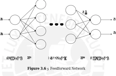
An artificial neural network forms when multiple of these neurons are connected and interchange their results. The easiest form to do this are feedforward multilayer networks, which can be seen in figure

𝑥1

𝑥2

𝑦1

𝑦2

Input-Layer 𝒘𝟏 _{Hidden-Layers 𝒘}𝐋 _Output-Layer

Figure 3.6 – Feedforward Network

There are three different types of layer in a multilayer network. The input layer takes in the data given to the network and provides them for the following layers. Therefore the number of neurons in this layer equals the number of inputs to the network. After the input layer follow any number of hidden layers, which absolve the computation of data. The final layer is called output layer and consists of as many neurons as the system has outputs to give them back at the environment. To compute data with the neural network, the data is given from layer to layer, which is called a forward pass. The output of every neuron in one layer is calculated before the processing in the next layer begins. Due to their ability to learn neural networks can be used in a variety of application, for example in modelling, speech/writing recognition or controllers. Their disadavantage is, that it is difficult to keep track on the learning process and ensure that the learned parameters are, in fact, correct ones.

3.2.2

Standard Backpropagation

An important step in the implementation of neural networks is the training. This describes the process of adapting the parameters in the network, so it will behave in the

𝑤L 𝑖𝑗

3 Foundations

2

−

desired way. One of the most basic ways to do this is error-backpropagation. The goal of this method is to adapt the weights at the connections between the neurons. This training method belongs to the techniques of supervised learning. These algorithms require that the desired output of the network is known so it can be compared to the real output. For the training process N pairs of input values (x) and desired output values, called teacher vector (t), are combined to a training set. The input values are presented to the network and the output is calculated via forward pass. The output can be written as a function of the input and the current network parameters (θ).

y = g(x, θ) (3.8)

The goal of training is to minimize the error of the whole training set

E(θ) = 1 i=1

(ti −g(xi, θ))2 (3.9) bybackpropagating it through thenetworkinanattempt toadjusttheweightresponsible for it. Therefore a gradient method is used: The weights are adapted in their proportion in direction of decline in the error

θk+1= θk+ ∆θ (3.10)

∆θ= ηδE

δθ (3.11)

In the second equation, ηis the learning rate, which determinates the size of steps made in the gradient direction. The derivative of E is computated via chain rule. For adapting the weight wijconnecting the j-th neuron in the L-th layer with the i-th neuron in the

(L + 1)-th layer it becomes

∂E ₌ ∂E∂yj ₌ ∂E ∂f(xj) ∂xj _(3.12) ∂wij ∂yj∂wij ∂yj ∂xj ∂wij

= δj dxj

dwij (3.13)

= δjyj (3.14)

where xjcthe combined input and yj= f (xjc) is the output of the j-th neuron in the

L-th layer. The δjin the last equation can be computed in a recursion with values from N

3 Foundations 𝑢𝑘 the (L + 1)-th layer. δj= ∂f(xj) w δ(L+1) (3.15) ∂xj k←j jk k

All these values will be available, as for backpropagation one starts at the output and work the way torward the input layer until all weights are adapted. With the δ-Notation, it is also often called Delta-Learning-Rule.

3.2.3

Dynamic Backpropagation

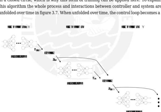
In chapter 3.2.2 the basic learning process of neural networks via backpropagation was explained. An extended method is dynamic backpropagation, which is explained in [5] andused for the training ofrecurrent neuralnetworks. This technique takes intoaccount that in this case information get fed back to the neural networks and works with this information from the past. When neural networks are used as controllers, they are also in a closed circle, which is why this form of training can be applied here. To explain this algorithm the whole process and interactions between controller and system are unfolded over time in figure 3.7. When unfolded over time, the control loop becomes a

𝑡𝑖𝑚𝑒 𝑠𝑡𝑒𝑝 𝑘 − 1 𝑡𝑖𝑚𝑒 𝑠𝑡𝑒𝑝 𝑘 𝑡𝑖𝑚𝑒 𝑠𝑡𝑒𝑝 𝑘 + 1 𝐶𝑜𝑛𝑡𝑟𝑜𝑙𝑙𝑒𝑟 𝑆𝑦𝑠𝑡𝑒𝑚 𝑥𝑘 𝐶𝑜𝑛𝑡𝑟𝑜𝑙𝑙𝑒𝑟 𝑆𝑦𝑠𝑡𝑒𝑚 𝐶𝑜𝑛𝑡𝑟𝑜𝑙𝑙𝑒𝑟

Figure 3.7 – Unfolded Network

series of repetition between the controller and the system. This means, that their errors 𝑢𝑘−1

3 Foundations

∂w

+

depend not only on the current parameters but also on past ones. Therefore for their value adaption, full derivatives until the starting point have to be calculated. This can be done in a recursive algorithm, which is explained below. The goal is to minimize the difference between the current and the desired position in every time step. This results in a cost function of

J = 1 (x1−x₁ ∗)2 + 1 (x2−x∗₂ )2 + ... + 1 (xN −x∗ )2 (3.16)

2 2 2 N

As before in standard backpropagation, the weights are adapted with

w_ij,(k +1) = wij,k −∆wij,k = wij,k −η ∂J

ij (3.17)

The overline in the last derivative signalizes, that the derivative is not only calculated to the actual influence, but is the total partial derivate considering all wijin the unfolded system. With equation 3.16 this total derivative can be split up to

∂J = N(x −x∗)∂xk (3.18)

The total derivative of xk is

∂wij k k=1 k ∂wij ∂xk ₌ ∂xk ∂xk ∂xk−1 _(3.19) ∂wij ∂wij ∂xk−1 ∂wij = ∂xk ₊ . ∂xk₊ ∂xk ∂uk−1Σ∂xk−1 _(3.20) ∂wij ∂xk−1 ∂uk−1 ∂xk−1 ∂wij

Leading to the recursive formular for computing the total derivative of the state to the weight in dynamic backpropagation for neural controllers:

∂x ∂x ∂u .∂xk+1 ∂xk+1 ∂ukΣ∂xk

k+1 ₌ k+1 k _{+ +} (3.21)

∂wij ∂uk ∂wij ∂xk ∂uk ∂xk ∂wij During training ∂xk+1

and ∂xk+1 are determined with the system model equations. ∂uk ∂uk ∂x_∂uk

The other derivatives - and

∂wij

k - are calculated by backpropagation through the ∂xk

controlling neural network.

3.2.4

Reinforcement Learning with an Actor-Critic-Algorithm

In the last two chapters techniques of backpropagation were explained as examplse of a supervised learning process. However, one may not always know the best value for the output of a network for comparison. For example in the case of controllers the desired

3 Foundations

state may be known, but not the value of the actuating variable to reach. Unsupervised learning techniques attempt to solve this problem. A group of these methods is called reinforcement learning. These algorithms let the network operate and observate how it influences the environment. If the result of the taken actions are satisfactional the positive feedback is given, otherwise a negative one. Information about reinforcement learning in general can be found in [6]

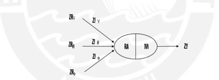
The reinforcement algorithm which is presented below is called ’Deep Deterministic Policy Gradient’ and was developed in [7]. It is based on [8] from 2014, in which the deterministic policy gradient was first presented. The algorithm was chosen because it can be employed for continuous state and action spaces, which are found in navigation problems. The algorithm has an Actor-Critic structure (see figure 3.8). The ’actor’ is

Figure 3.8 – Structure of an Actor-Critic network

the network which shall be trained. Based on a policy µa(s), it decides which action a is taken in a specific state s. A deterministic policy can simply be seen as the actor network with its current structure and parameters, computing an action as an output.

ak= µa(sk) (3.22)

The action akeffects the environment and an immediate feedback is given in form of a reward rk. The reward can be positive or negative, depending on weather akhelped the system to reach a defined ojective. An ideal policy µ∗_{a would chose actions which lead to} the highest accumulated reward R in a long term horizon. To adapt the current policy in the direction of the ideal policy another network is employed, the so-called ’critic’. It evaluates the taken action in every time step by estimating the action-value function

Q(s, a), which represents the expected long-term reward if action a is taken at state s. 𝐴𝑐𝑡𝑜𝑟 𝑎𝑐𝑡𝑖𝑜𝑛 𝑃𝑜𝑙𝑖𝑐𝑦 𝑉𝑎𝑙𝑢𝑒 𝐹𝑢𝑛𝑐𝑡𝑖𝑜𝑛 𝐶𝑟𝑖𝑡𝑖𝑐 r𝑒𝑤𝑎𝑟𝑑 𝑠𝑡𝑎𝑡𝑒 𝐸𝑛𝑣𝑖𝑟𝑜𝑛𝑚𝑒𝑛𝑡

3 Foundations

The ascending gradient of this function leads in the direction of the ideal policy and is therefore used for adapting the current policy. The problem is, that the action-value function is not known in the beginning and the critic network has to learn it. The ideal action-value function returns the highest accumulated reward to be expected under the current policy:

Q∗(_sk,ak) = _maxµ

aE[R|sk,ak] (3.23) This optimal function fullfills the so-called Bellmann equation

Q∗_{(sk,ak) = E[rk + γQ}∗_{(sk+1,ak+1)] (3.24)} with γbeing a discount factor between 0 and 1. The ideal value can be calculated with this equation and the difference to the current output can be backpropagated through the critic network. As the action value Q∗(_{sk+1, ak} + 1) _{and therefore the action ak+1} of the next time step is needed, two additional networks are implemented. These are called target networks and estimate the future values. With the parameters of the actor and critic networkbeing θaand θcthe target networks parameters are designed to slowly follow them and updated via

θat = τθta + (1 −τ)θta θct = τθtc + (1 −τ)θtc

(3.25) (3.26) with τ << 1. Th outputs of the target networks can then be defined respectively as

µt (_{sk+1, ak} + 1_{, θ}t ) _{and Q}t(_{sk+1, ak+1, θ}t) _{With these information it is possible to train}

a a c

the actor and critic network as described below for the time step k. The loss function at the critic network output is constructed with the mean square error

L(θc) = E[(rk+ γQt(sk+1, ak+1) −Q(sk, ak, θc))2] (3.27) The critic network is adapted with the gradient to its parameters

∂L(θc) = _E[(r + γQt(s , a ) −Q(s ∂Q(sk, ak, θc) ∂θc k θc = θc + ηc∂L(θc) ∂θc k+1 k+1 k, ak , θc)) _∂θc ] (3.28) (3.29)

3 Foundations

The parameters of the critic network are updated with the gradient of the action-value function:

∂Q(sk,ak, θa) = ∂ Q(sk, ak, θa) ∂ak _(3.30)

∂θa ∂ak ∂θa

θa = θa + ηa∂Q(sk, ak, θa)

∂θa (3.31)

As the estimated policy is deterministic it does not explore on itself. This means the actor choses the same action in the same situation every time. As it is necessary to try different actions in order to find the best policy a random process is added as a noise to the taken actions to ensure sufficient exploration. In [7] an Ornstein-Uhlenback random process is named to be suitable for this kind of task. As the random values generated by this process are temporally correlated they let the actor explorate efficiently in one direction.

In practice there are difficulties with updating the networks every time step with the new information, which are rooted in the temporal dependence of the incoming data. This is why [7] proposes to let the actor sample transitions in a form like (sk, ak, rk, sk+1)

and store them in a replay memory. For learning some samples from the replay memory are randomly chosen in a minibatch for learning.

3.3

Fuzzy Neural Networks

Fuzzy neural networks are hybrid systems of the both mentioned structures. The idea is to model a fuzzy inference system as a neural network. The parameters of the system can then be adapted by employing learning strategies. This kind of architecture was first presented in [9] as an ’Adaptive-Network-Based Fuzzy Inference System’ (ANFIS). For explaining the functionality a system with 2 inputs(x1 and x2 ), 1 output(yˆ) and

two rules is considered. The fuzzy sets for the input are A1 and A2 for x1 and B1 and

3 Foundations 𝐿𝑎𝑦𝑒𝑟 1 𝐿𝑎𝑦𝑒𝑟 2 𝐿𝑎𝑦𝑒𝑟 3 𝐿𝑎𝑦𝑒𝑟 4 𝐿𝑎𝑦𝑒𝑟 5 𝑥1 𝑦ො 𝑥2 Figure 3.9 – Fuzzy-Neural-Network

The fuzzy neural network consists of 5 layers in a feed-forward structure containing different types functions.

The nodes in the first layer contain the membership functions and take over the task of fuzzification. Note that because the networkshall be trained, the membership functions need to be at least piecewise differentiable. Thus the proposed fuzzy membership func- tions (see chapter 3.1.1) can be employed here but are nevertheless often approximated with other, differentiable functions. For instance the triangle shape can be expressed with a gaussian function

−(x−c)2

µ(x) = e a and the ramp with a sigmoid function

µ(x) = 1 + 1 e a

−x−c

The variables c and a are different for everymembership function as they determine the center (c) and slope (a) of the function. From the view of fuzzy systems they define the position and size of the fuzzy sets for the input space. These parameters are called

’premise parameters’ and are adaptable during training.

The second layer realizes the aggregation of the premises by using AND-operators in the nodes. In the figure above the AND is realized with a product. The result of this

𝐴1 𝑥1 , 𝑥2 Π 𝑁 𝑓1 𝐴2 ∑ 𝐵1 Π 𝑁 𝑓2 𝑥1 , 𝑥2 𝐵2

3 Foundations

z =

layer for rule i is called ’firing strength ziof rule i’.

zi = µAi · µBi

The third layer contains normalization nodes. They scale the firing strenghts by dividing it by thesumofall firing strengths. The outputs of this layerarereferred toas’normalized

firing strengths’. This step realizes the easy defuzzification for Takagi-Sugeno fuzzy systems, described in 3.1

N zi

i _z

1 + z2

The fourth layer calculates the rules cosequences and represents the inference from FIS. As ANFIS is based on Takagi-Sugeno fuzzy systems, the rules have linear combinations of the input variables as consequences.

IF A1 AND B1 THEN f1 = p1x1 + q1x2 + w1

IF A2 AND B2 THEN f2 = p2x1 + q2x2 + w1

As every rule should be active in the same way their premise is active, the consequences are multiplied with the normalized firing strengthes.

zN _fi = _zN (_pix1 + _qix2 + _wi)

i i

The parameters pi, qiand wi are called ’consequence parameters’ and can be changed by training to adapt the network.

The fifth and last layer concludes all rules consequences into one output by adding them up. The final output is therefore:

yˆ = Σ _z ifi zN _fi = i i Σ _z i i i

Fuzzy-Neural-Networks combine the advantages of fuzzy and artificial neural systems. The structure and functionality is easily comprehensible and can be set up without problem with parameters from expert knowledge. By having the possibility to change parameters with a training sequence the system can learn and adapt.

3.4

Neuro-Fuzzy-Control in Robot Navigation

Hybrid networks with fuzzy and neuralelements havebeensuccessfully implemented in many systems for control purposes. The applications range from the control of household

3 Foundations

devices like washing mashines [10] to process control in power plants [11]. Another branch benefiting from neuro-fuzzy-techniques is the field of autnomous mobile robots. Fuzzy neural controllers can help to tackle the challenges of navigation and obstacle avoidance, and have therefore been employed several times for these tasks.

In [12] an ANFIS-Controller was developed for the navigation of a mobile service robot with two differential wheels. It was trained to recognize and follow a line on the floor to its goal position. To realize this the desired motor speed values were predefined in a teacher vector. The fuzzy controller was then adapted in premise and consequence parameters of the rule base via supervised learning and could eventually lead the robot along the line. An approach for an obstacle avoidance controller is given in [9], where a two-wheeled robot should be able to move in a fixed area without colliding with the objects lying within. The parameters of the membership functions and the consequence part were adpated with supervised learning. The controller was tested in simulation and also experimentally. The authors in [13] focused on the adaption of the parameters in the membership functions. They predefined all parameters and set a perfect route to a goal position without colliding with an obstacle. This path was then used for adapting position and slope of the membership functions to "smooth the trajectory generated by the fuzzy logic model". The controller was employed sucessfully in a two wheeled, differential driven robot. To decrase the number of rules in one fuzzy controller the navigation algorithm in [14] is split up in a hierarchial system. Within this, different behaviours like e.g. "goto-target" or "turn-corner" are realized with respective neuro-fuzzy controllers. By doing this they could avoid having one big rule base to include all navigation orders.

Reinforcement approaches for the navigation problem were taken in [15], with using adapted versions of Q-Learning and Sarsa-Learning algorithms. Another example is [16], where a controller for line following of a two wheeled, differential driven robot could be developed and tested in simulation. A 4-wheeled non-holonomic car-type robot, like the one considered in this thesis is the subject in [17]. A neural fuzzy controller was trained with a supervised training algorithm to find its way to a goal position and avoid obstacles in its path. The controller was implemented in a real experiment environment and could successfully drive to the target point without colliding with any objects. The paper [1], which builds the foundation for this thesis, describes the developement of a neural fuzzy controller for navigating a 4-wheeled robot from differentstarting positions and angles in a goal parking position. The goal for this thesis is to develop the existing controller further and add the ability to avoid obstacles.

Chapter 4

Implementation

4.1

Model

For the development of the navigation algorithms a model of the system was needed. Figure 4.1 shows the robot considered in this work. The two back wheels are fixed and connected to the motor to provide the traction while the two front wheels are steerable. At any time the state s of the robot is defined by its position and orientation in the ground coordinate system. The position is described by its x- and y-coordinate and the orientation by the angle φ .

xk

sk= yk (4.1)

φk

The model should describe the dynamical transition of the robots state from one time step to another based on the actual state and the steering angle δ as the control input. The kinematic equations of cartype-mobile robots are derived in [1]. With the robot moving backwards and only a very small, fixed distance r every time step the model results in xk+1 = xk+ rcos(φk) (4.2) yk+1 = yk + rsin(φk) (4.3) r φk+1 = φk− _Ltan(δk) (4.4) (4.5)

4 Implementation

𝑦

𝑦𝑝

𝑥𝑝 𝑥

Figure 4.1 – 4-wheeled car-type robot

where L the length of the robot measured between the front and back wheels and δk the current steering angle input. The steering angle is restricted to −30◦_{< δ < 30}◦ This model applies for a slow motion of the robot at constant speed. Also it doesn’t

consider slipping and skidding of the wheels.

4.2

Navigation

4.2.1

Structure of the Neuro Fuzzy Controller

The strategy for solving the problem is to let the robot move to the position of x∗_{= 0} while reaching the desired orientation of φ∗₌

2π. After that position is reached, the

robot will just move straight in positive y-direction and the control variable will be δ = 0◦_{. It can be seen in figure 4.2 that the taken path is independent of the robots y-} position. Therefore the controller does not need the y position to determine the steering angle and uses only the x-position and the angle as inputs. As long as there is enough space in y-direction the robot will be able to reach its goal with this information. From here on the position in x-direction and the orientation of the robots are concluded in the state-vector s:

s_k = Σxk Σ φk

(4.6) The structure of the Neuro-Fuzzy-controller is given in figure 4.3. It has the same 5 layers as the standard neuro fuzzy system described in 3.3. The only difference is, that the controller usedhere is basedonazero-order Takagi-Sugeno fuzzy system. Therefore

𝛿

4 Implementation

𝑦

−50 0 50 𝑥

Figure 4.2 – Strategy to reach the goal position. The control input does not depend on the y-position of the robot, only on the x-position and orientation.

the consequences are not a linear combination of the inputs, but reduced to one single value wiper rule.

Seven membership partitions were used for each of the 2 inputs. The initial membership functions used for x and φ can be seen in figure 4.4. Table 4.1 lists their center and slope values as well as the respective linguistic interpretation. The outer Membership- functions of the position are sigmoid functions, because for every x-value smaller then

−50/greater than 50 the steering command should be full right/full left, the same as at

−50/50. The outer membership functions of the orientation are gaussian, because the an- gle range is only 2πand the value at the left end is the same as the value at the right end.

cx ax linguistic interpretation cφ aφ linguistic interpretation

1 2 3 4 5 6 7 −50 −34 −13 0 13 34 50 4 10 6 3 6 10 4 FAR LEFT LEFT CLOSE LEFT ZERO CLOSE RIGHT RIGHT FAR RIGHT -1.042 -0.2618 0.9599 1.5708 2.1817 3.4034 4.1888 0.1745 0.3491 0.3491 0.0524 0.3491 0.3491 0.1745 DOWN RIGHT RIGHT UP RIGHT UP UP LEFT LEFT DOWN LEFT

Table 4.1 – Initial center and slope parameters as well as linguistic interpretation of the membership functions for the navigation control system

4 Implementation Π 𝑁 𝑤1 𝑧1 𝑧𝑁 ₁ 𝑧_𝑠𝑢𝑚 Π 𝑁 𝑤2 𝑧2 𝑧₂ 𝑁 𝑧_𝑠𝑢𝑚 𝛿 ∑ Π 𝑁 𝑤80 𝑧48 𝑧 ₄₈ 𝑁 𝑧_𝑠𝑢𝑚 Π 𝑁 𝑧49 𝑤₈₁ 𝑧 𝑁 49 𝑥 𝜙 𝑧𝑠𝑢𝑚

Figure 4.3 – Structure of the Neuro Fuzzy Controller

Figure 4.4 – Initial membership functions of the x-position (above) and the ori- entation φ (below)

The results of the membership functions are aggregated by using the product as a fuzzy AND-operator. The results are the premises z1 · · · z49. These are normalized in

the next layer as a part of the defuzzification.

zN ₌ zi _(4.7)

zsum i

4 Implementation

k

k

c _k

with z = Σ49 z . Afterwards the normalized premises are multiplied with their

sum

j=1 j

respective weight wito determine the results of theirs rules. In the final step all of the results are added up to form the steering angle output. Because of the normalization step every weight wigets as much power on the output as their premise was active.

4.2.2

Training with Dynamic Backpropagation

The navigation controller was trained with dynamic backpropagation as described in chapter 3.2.3. The whole training process is listed in algorithm 4.1 and will be explained further here.

At first the vectors with the slopes (a) and centers (c) of the membership functions as well as of the rules consequences (w) are initialized. Five symmetric starting states are defined as well as the maximum of training episodes.

One training episode consist of following all starting positions for 1350 time steps or until the path leaves the field boundaries of xmin = −50 and xmax= 50. The network parameters are updated after every episode with the ratio of the sum over all calculated changes from the timesteps in this episode to the number of time steps included in this sum (ktotal). k_Σtotal i,k wi = w_i −ηk=1 total k_Σtotal ∆a (4.8) ai = a_i −η_a k=1 total k_Σtotal ∆c i,k (4.9) i,k ci = c_i −η k=1 total (4.10) In each time step k the current state sk is fed to the controller, which computes the

steering angle uk = δk with the available parameters. The steering angle is given to the model of the system, which calculates the next state sk+1 = fm(sk, uk) with the kinematic equations from 4.1. This position is compared with the desired position and the error ek is determined.

ek = Σ x_k+1 −x∗Σ φ_{k+1 + φ}∗

With the error and the equations from the dynamic backpropagation algorithm, the gradient toadapttheparameters canbe calculated. Belowtheequations for adapting the

4 Implementation 2 ∂w L ∂ k ∂uk L k =

a rule consequence parameter wiin the navigation controller will be derived. Differences fo the derivation of the equations for the premise parameters will be listed afterwards. As explained in chapter 3.2.2, the rate of change is the total derivative of the cost function to the parameter. For consequence i that is

∆wi = ∂J ∂wi

The cost function to minimalize consists of the error to the desired state.

(4.11)

J = 1 (sk+1−s∗)2 (4.12)

With the application of chain rule the total derivative becomes ∂J

∂wi

= (sk+1−s∗) ∂sk+1

i

(4.13) As derived in chapter 3.2.2 this is calculated in a recursive way:

∂sk+1₌ ∂ sk+1₊.∂sk+1₊ ∂sk+1∂ukΣ ∂sk

∂wi ∂wi ∂sk ∂uk ∂s

k ∂wi

(4.14)

∂sk+1

∂wi is split up by applying the chain rule. The first derivative is then calculated from

the system model, the second from the controller structure:

Σ

∂sk+1 ₌ ∂sk∂uk _{= 0}

Σ

zN _(4.15)

∂wi ∂uk∂wi −r i

The next two derivatives are constructed as well with the help of the system model ∂s ∂ xk+1 ∂xk+1 Σ 1 _r · _cos(_φ Σ k+1 ₌ ∂sk ∂sk+1₌ ∂uk ∂xk ∂φ_k+1 ∂xk ∂xk+1 ∂u φk+1 ∂φ k) ∂φk+1 ∂φk Σ Σ 0 = −r (4.16) (4.17) 0 1

4 Implementation

j

= z

For the last derivative the structure of the controller is used again. ∂uk₌ ∂s ∂uk ∂xk (4.18) ∂uk ∂φk ∂ uk ∂ 49 N ₌ 49 ∂zN _(4.19) w ∂xk ∂xk j=1 wjzj j=1 j ∂xk ∂uk ₌ ∂ 49 ∂zN (4.20) j N _{= w} ∂φk ∂φk j=1 wjzj j=1 j ∂φk

To compute the derivative of the normalized premises, the product rule has to be used. ∂zN ∂zj _z sum −zj ∂zsum j ∂xk ∂xk 2 _sum ∂xk (4.21) ∂zN ∂z_{j z} sum −zj ∂zsum j ∂φk = ∂φk sum 2 ∂φk (4.22) The derivatives of the unnormalized premises and their sum are

∂zj ₌ ∂µx,1 _{(µ 1}w1 +µ 2w2 +· · · + µ 7w7)+ (4.23) ∂xk ∂xk φ, φ, φ, ∂µx,2 _{(µ 1}w8 +µ 2w9 +· · · + µ 7w14) + · · · ∂xk φ, φ, φ, ∂µx,7 _{(µ 1w}43 +µ 2w44 +· · · + µ 3w49) ∂xk φ, φ, φ, ∂zj ₌ ∂µφ,1 _{(µ w} + µ w + · · · + µ w )+ ∂φk ∂φk x,1 1 x,2 2 x,7 7 ∂ µφ,2 _{(µ w} + µ w + · · · + m w 4) + · · · ∂φk x,1 8 x,2 9 7 1 ∂ µφ,7 _{(µ w} + µ w + · · · + µ w ) (4.24) ∂φk 4 x,1 43 x,2 44 x,7 49 ∂zsum _{= 9} ∂zj _(4.25) ∂xk j=1 ∂xk 4 ∂zsum _{= 9} ∂zj ∂φk _j=1 ∂φk (4.26) k = 49 z

4 Implementation

The derivatives of the membership function to the input depend on the type of function used. For the sigmoid functions it is

∂µx,i _{= −}1 _µ

x,i(x )(1 −µx,i (x )) (4.27)

∂xk ai k k

and for the gaussian funtions it results in ∂µx,i _{= 2 (x}

k −c )µ (x ) (4.28)

∂xk ai i x,i k

With all derivatives from the update equation broken down in terms which can be taken directly from the model or the controller, the change of consequence parameters can be calculated in every time step.

The derivatives to update the premise parameters are calculated analog except for 4.27 and 4.28, which are

∂µx,i _{= −}1 _µ

x,i(x )(1 −µx,i (x )) (4.29)

∂ci ai k k

∂µx,i _{= −}1 (_x −c )µ (x )(1 −µ (x )) (4.30) ∂ai

for sigmoid functions and

a 2 k i i x,i k x,i k ∂ µx,i _{= 2 µ} x,i (x )(x −c ) (4.31) ∂ci ai k k i ∂ µx,i _{= 1 µ} (x )(x −c ) (4.32) for gaussian functions.

∂ai a _{2 x,i k k i} i

In the navigation controller the premise parameters, as well as the consequence pa- rameters can be chosen symmetrically, as the strategy to reach the desired position is mirror-inverted to the middle lane. Therefore in updating the parameters only one half is used and projected on the other half of the parameters. As the starting states are chosen to symmetrical, no information is lost.

The parameters of the slopes and centers had to be restricted. Especially the slopes would rise and lead to an overlapping of all membership function. That is there are maximum and minimum limts for components of the a- and c-vector.

The learning rates were desingned to be slightly adaptable. A simple system was chosen in which every parameter has its own learning rate. If the parameter is to be adapted in the current episode in the same direction (positive ornegative) as in the lastepisode, the

4 Implementation

learning rate increasing with the factor 1.1 If the directions are different, the learning rate will be decreased by 0.5. For every parameter vector a maximal rate is defined to avoid that rates swing up fast and make the learning process instable. In general the learning rates had to be chosen very small.

Forthe training with dynamic a technique called "incremental learning" was employed. This means at the beginning of training starting positions close the the goal position (in x-position and angle) were used. When parameters for these were learned with success the starting positions were chosen to become more and more difficult. Accordingly, the algorithm 4.1 is to run numerous times with changed starting parameters for approx- imitaly 1000 episodes. This way it can be made sure the algorithm learns the correct steering technique, with the possibility to check after every learning stage.

4 Implementation

k

1: Initialize premise parameter vectors a and c and vector with rule consequences w 2: Set symmetric starting points for training s0,1 · · · s0,M

3: for each episode i do

4: for each starting position j do 5: for each time step k do

6: Compute control signal uk= fc(xk, φk)

7: Apply uk to model and compute state in next time step sk+1 = fm(sk, uk)

8: Caluclate error to desired position ek= sk− s∗

9: Compute total derivatives with equations 4.14 - 4.32 10: Calculate weight changes and them up

∆sumw = ∆sumw + e ∂sk+1 ∂w ∆sumc = ∆sumc + ek∂sk+1 ∂c ∆sum a = ∆sumw + ek∂sk+1 ∂a 11: end for 12: end for

13: Calculate changes of parameters

∆w = ∆sumw k_total ∆c = ∆sumc ktotal ∆a = ∆suma ktotal

14: Update step sizes

15: Update weights and premise parameters

w = w −ηw∆w

c = c −ηc∆c

a = a −ηa∆a

16: Restrict premise parameters and mirror all parameters 17: end for

Algorithm 4.1 – Training the neuro fuzzy navigation controller with dynamic backpropagation

4 Implementation

4.3

Obstacle Avoidance

4.3.1

Structure of the Neuro Fuzzy Controller for Obstacle Avoidance

The idea was to design an additional neural fuzzy controller for obstacle avoidance. It generates a variable δplus which is added to the steering angle δ of the navigation controller. With this manipulation thesteering angle is adpated if anobstacle is detected. A diagram of the control cycle with two controllers can be seen in figure 4.5. The

Figure 4.5 – Control cycle with Navigation and Obstacle Avoidance Controller

structure of the obstacle avoidance controller is again in 5 layers as described in 3.9 and can be seen in figure 4.6

(𝑥𝑐; 𝑦𝑐) 𝑂𝑏𝑠𝑡𝑎𝑐𝑙𝑒 𝐴𝑣𝑜𝑖𝑑𝑎𝑛𝑐𝑒 𝐶𝑜𝑛𝑡𝑟𝑜𝑙𝑙𝑒𝑟 𝛿𝑝𝑙𝑢𝑠 + 𝑁𝑎𝑣𝑖𝑔𝑎𝑡𝑖𝑜𝑛 𝐶𝑜𝑛𝑡𝑟𝑜𝑙 𝛿 𝑅𝑜𝑏𝑜𝑡 𝒔

4 Implementation Π 𝑁 𝑤_𝑜,1 𝑧_{𝑜,1 𝑧}𝑁 𝑜,1 𝑧𝑜,𝑠𝑢𝑚 Π 𝑁 𝑤_𝑜,2 𝑧 _𝑜,2 𝑧𝑁 𝑜,2 𝑧𝑜,𝑠𝑢𝑚 𝛿𝑝𝑙𝑢𝑠 ∑ Π 𝑁 𝑤𝑜,133 𝑧_𝑜,133 𝑧𝑁 𝑜,133 𝑧𝑜,𝑠𝑢𝑚 Π 𝑁 𝑤𝑜,134 𝑧𝑜,134 𝑧𝑁 𝑜,134 𝑧_{𝑜,𝑠𝑢𝑚} Π 𝑁 𝑤𝑜,135 𝑧_𝑜,135 𝑧𝑁 𝑜,135 𝑑𝑖𝑠𝑡𝑙 𝑑𝑖𝑠𝑡𝑟 𝑑𝑖𝑠𝑡𝑓 𝑎𝑛𝑔𝑙𝑒𝑔 𝑧𝑜,𝑠𝑢𝑚

Figure 4.6 – Structure of the controller for obstacle avoidance

The input variables for the controller are the detected distance to an object on the left, front and right of the robot and the current orientation angle of the robot. The membership functions for the input can be seen in figure 4.7, the chosen parameter values and their liguistic interpretation in table 4.2. The output is the manipulation variable δplus, which corrects the steering angle from the navigation controller to avoid obstacles.

cl al linguistic interpretation cg ag linguistic interpretation 1 2 3 4 5 1 4 7 1 3 0.5 TOO NEAR NEAR FAR −34 π −π₄ 0 π 4 3π 4 0.3491 0.3491 0.3491 0.34914 0.34914 DOWN RIGHT UP RIGHT UP UP LEFT DOWN LEFT

Table 4.2 – Initial center and slope parameters as well as linguistic interpretation of the membership functions for the obstacle avoidance control system. The parameters are the same for the three distance inputs.

4 Implementation 4 4 1 Distance Left 0.5 0 -5 0 5 10 15 20 1 Distance Right 0.5 0 -5 0 5 10 15 20 1 Distance Front 0.5 0 -5 0 5 10 15 20 1 Orientation 0.5 0 -4 -3 -2 -1 0 1 2 3 4

Figure 4.7 – Membership-Functions of the Obstacle Avoidance Algorithm

4.3.2

Simulation of Obstacle Recognition

The next step was to design a simulation for the recognition of obstacles, which would provide the distance between robot and object as if it was measured. Circular objects were chosen for this simulation because in that case the distance between robot and object is easily computable with the following equation

.

distc= (xc−x)2 + (yc−y)2 −R (4.33) where (xc; yc) are the center coordinates of the cicular object and R is its radius. Additionally to the distance it needs to be decided if the obstacle is on the left, right or front of the robot. The angle to the center of the obstacle is determined with the equation

β _c = arctan((yc − y)) −π (4.34)

xc−x 2

The standard value for the three distance inputs is 100, symbolizing that the path is clear. This value is overwritten by the distance to the object if the angle to the object

falls into the following ranges:

−π < βc < −π → Object left, distl= distc

2 8

π _{< β}

c < π → Object front, distf= distc