* Corresponding author. Tel: +98(21) 7322-5067 Fax: +98(21) 7322-5098 E-mail address: [email protected] (S. M. Sadatrasou)
© 2015 Growing Science Ltd. All rights reserved. doi: 10.5267/j.dsl.2014.9.005
Decision Science Letters 4 (2015) 35–50
Contents lists available at GrowingScience
Decision Science Letters
homepage: www.GrowingScience.com/dsl
An application of data mining classification and bi-level programming for optimal credit allocation
Seyed Mahdi Sadatrasou*, Mohammad Reza Gholamian and Kamran Shahanaghi
School of E-commerce and Industrial Engineering, Iran University of Science and Technology, Tehran, Iran
C H R O N I C L E A B S T R A C T Article history: Received March 15, 2014 Accepted September 6, 2014 Available online September 9 2014
This paper investigates credit allocation policy making and its effect on economic development using bi-level programming. There are two challenging problems in bi-level credit allocation; at the first level government/public related institutes must allocate the credit strategically concerning sustainable development to regions and industrial sectors. At the second level, there are agent banks, which should allocate the credit tactically to individual applicants based on their own profitability and risk using their credit scoring models. There is a conflict of interest between these two stakeholders but the cooperation is inevitable. In this paper, a new bi-level programming formulation of the leader-follower game in association with sustainable development theory in the first level and data mining classifier at the second level is used to mathematically model the problem. The model is applied to a national development fund (NDF) as a government related organization and one of its agent banks. A new algorithm called Bi-level Genetic fuzzy apriori Algorithm (BGFAA) is introduced to solve the bilateral model. Experimental results are presented and compared with a unilateral policy making scenario by the leader. Findings show that although the objective functions of the leader are worse in the bilateral scenario but agent banks collaboration is attracted and guaranteed.
© 2015 Growing Science Ltd. All rights reserved.
Keywords:
Bi-level programming Classifier
Sustainable development
1. Introduction
Governments and public sectors intervene in financial markets to promote the industrial development is one of the distinguishing characteristics of developing countries transitional economy (Xiuli, et al., 2012). In recent years, there has been a great interest in credit allocation problems in developing countries because of its impact on overall development and competitiveness of their economies (Firth et al., 2009). There are some studies, which indicate that credit controls the investment and development activities of companies (Leite & Vaez-Zadeh, 1986). Commercial banks have long been active participants in financial markets and thus any credit allocation policy should do with their cooperation as the agents and could influence on their profitability and risk. The mentioned economic environment shapes an application of credit allocation with two decision modeling steps, which are connected in a hierarchical way, the upper the leader and the lower the follower. Since the decision
makers in each level have their own policies of credit allocation, mutually conflicting objective and constraint are not unexpected. This situation can be seen in supply chain networks, taxation, setting penalties for illegal drug import, etc. and usually they are modeled using bi-level programming in different studies (Bard et al., 2000; Lee & Shih, 2000; Ryu et al., 2004).
The problem faced by the government/public sector institutes in the first level is to determine the credit allocated to various industrial sectors/regions in order to maximize return and minimize the risk considering sustainable development at the country level. On the other side, in the second level, the agent banks look for minimizing the credit risk of their applicants. The secondary objectives of them could be the profitability of the applicants and ease/cost effectiveness of credit scoring process. The conflict inherent in the problem is that the first level wants to maximize its profit and minimize its risk at industrial sectors level subject to a given level of sustainable development while the second level wishes to minimize its credit risk and maximize profit subject to a given ease of scoring process. The credit allocation scenario can be viewed as a leader-follower Stackelberg game in which the former sets policy and the latter reacts, sometimes with unforeseen consequences. The government decisions can be modeled using a linear programming model (Markowitz, 1952). The agent banks use the credit scoring in order to evaluate their loan applicants (Gholamian et al., 2012; Thomas, 2000). Credit scoring usually classifies loan applicants in terms of good and the bad ones. There are many techniques introduced in the literature, including data mining and mathematical programming approaches. Data mining methods such as neural networks, support vector machines, Bayesian networks, case based reasoning, decision trees are superior to other approaches in many studies, apriori (Harrell & Lee, 1985; Thomas, 2000).
As explained, the study inevitably is faced with a combination of operation research (OR) and data mining (DM) techniques. Three types of synergies are distinguished between operation research and data mining in the literature:
OR to increase DM efficiency,
DM to increase OR effectiveness by replacement,
DM to increase OR effectiveness by refinement.
In fact, from one side, optimization methods increase data mining efficiency and from the other side, data mining increases effectiveness of operation research (Meisel & Mattfeld, 2010). The study uses the second approach for model formulation as modeling the papers credit scoring model in a mathematical programming approach and faces many problems because of nonlinearities and big problem scale. This paper approaches the second scenario using a data mining classifier in bi-level programming, which is not mentioned in the previous studies. The approach uses data mining in order to increase the effectiveness of bi-level programming by replacing a fuzzy apriori classifier with a mathematical programming shape of credit scoring, which has numerous nonlinear problems (Thomas et al., 2002). This study is divided into six major parts: section 2 describes the basic concepts. Section 3 introduces the general bi-level credit allocating model. Section 4 describes decision making process and the new BGFAA algorithm. Experiments, results and discussions are presented in section 5 and finally, study concluded in section 6.
2. Basic Concepts of the Hybrid OR/DM Bi-level Credit Allocation Model
In this section, basic concepts used for building general bi-level credit allocation model are described in brief.
2.1Bi-level programming
Historically, bi-level programming is a kind of Stackelberg games (von Stackelberg, 1952). In Stackelberg, game agents interact at two different levels, which are mainly leader and follower, usually the leader determines the directives for the follower. Mathematically, the leader chooses the x
strategy and the follower i chooses the set of yi strategies. A bi-level programming problem (BLPP)
can generally formulated as (Colson et al., 2005): min , ∈ , . . , 0 min , . . , 0 (1)
where ∈ and ∈ . The variables are mainly divided into two various classes x and y, which
are orderly the upper and the lower variables. Also, the functions F: × → R and f: ×
→ R are the upper-level and lower-level objective functions and the constraints G: × → R
and g: × → R are upper-level and lower-level constraints, respectively. The sequential nature
of the decision implies that y is a function of x (Bard, 1998). There are also some usual investigations
that for all decisions taken by the leader, there are some remained feasible space for the follower (Bard, 1998). There are several problems, which can be modeled using bi-level programs, these problems mainly investigate the challenges of the two decision makers where the decisions are hierarchically interrelated and this relationship influences on the utilities of both players. There are so many applications of the mentioned concept in different areas including management, economic planning, engineering, chemistry and etc. (Colson, et al., 2005).
2.2Interval Linear Programming
In mathematical programming objective functions and constraints coefficients are usually described by crisp values sets. When the decision maker faces uncertainties, there are some alternatives including fuzzy, stochastic, interval and other approaches; each of which has its own characteristics. In financial asset allocation, interval programming is a favorite approach for modeling uncertainty. This usually takes place because the decision maker is not easy to specify membership functions or the probability distributions. In these situations, the intervals help decision maker include his/her purpose in the model an interval can be shown as (Sengupta et al., 2001):
, ∈ : , (2)
where , are the left and right limits of interval A on the real line, respectively. If these two limits where equal then A becomes a real number. All coefficients of objective functions and constraints can
be modeled using intervals but they depend on the nature of the problem. There are different methods introduced to solve linear interval programming but this paper uses the method in which seeks to change it to a kind of crisp mathematical problem (Sengupta, et al., 2001).
2.3Balancing the Data
Building classifiers on imbalanced data has many problems, including over fitting and having poor rate of learning. In general, the more the balance between good and bad ones, the more accurate the resulting score is (Finlay, 2011). Real credit scoring datasets are often imbalanced because the number of bad applicants is often fewer than the number of good ones. This study uses a real world Iranian credit dataset in; therefore, data balancing must be taken into consideration. There are different data balancing techniques including random over sampling, random under sampling, model based and stratified; each of them has its own strengths and weaknesses. This paper uses the random oversampling method in order to balance the data.
2.4Sustainable development
Economic development has different challenges and effects on the society, environment and other aspects of human life. Sustainable development is a theory and philosophy to overcome and to manage these challenges of development in long term and it is the focal area of attentions for
countries, especially the developing countries. There are some indicators in the literature to evaluate the sustainability of development. There are 440 indicators extracted for evaluating various aspects of sustainable development on the works accomplished by United Nations department of Economic and Social Affairs (Economic, 2007). There are also other studies introduced the indicators for a special vertical industries for example energy sector (Streimikiene et al., 2007). This paper introduces the general bi-level credit allocation model subject to sustainable development, but lacking appropriate data forced it implementing selected indicators in the final model rather than the whole.
2.4.1 Comparative advantage
Comparative advantage is the ability of a country to produce something at the lower opportunity and marginal costs (Hunt & Morgan, 1995). The revealed comparative advantage (RCA) is a popular measure used to calculate the comparative advantage in a particular class of goods or services. Balassa presented an advanced measure (index) of RCA later (Utkulu & Seymen, 2004). This is a widely accepted in the literature and it is expressed as Eq. (3) (Utkulu & Seymen, 2004):
BIRCA= (Eij / Eit) / (Enj / Ent), (3)
where E represents exports, i is a country, j is an industry, t is a set of industries and n is a set of
countries. RCA measures a country’s exports of an industry relative to its total exports and to the exports of a set of countries, e.g. the world. If BIRCA>1 a comparative advantage is “revealed” and
one can say that the ith country has comparative advantage against Asia reign, for instance. If BIRCA is
less than one, the ith country is said to have a comparative disadvantage in that industry sector against
continent. Laursen discussed on revealed comparative advantage as a measure of specialization in economics, he also discussed to normalizations of the original index and finally proposed an alternative and more traditional strategy in order to analyze the dynamics of specialization as described in Eq. (4) (De Benedictis & Tamberi, 2001; Laursen, 1998).
LRCA= (BIRCA-1)/ (BIRCA+1) (4)
This index ranges from -1 to +1 and it is therefore symmetric. If LRCA>0a comparative advantage is
“revealed” and If LRCA< 0 there is the comparative disadvantage. In this paper, LRCA is used with
some modifications in the original formula and can be defined as Eq. (5):
and for Ltg: Ltg= (BItg-1)/ (BItg+1)
(5)
2.4.2 Population work culture
From the native economy analysis, the region’s economy can be divided into basic and non-basic industry sectors. Basic industries are those exporting to other regions and bringing wealth from them; non-basic industries support basic industries in the region. Often the work culture of the country economy is based on the basic rules and the population can have unofficial relations among social networks in order to synergize their capabilities. Location quotient is used as a popular measure for LQ, which can be defined by Eq. (6):
6
where Jtg represents total amount of employment (jobs) in industry sector t in gth region.
∑ represents total g regions’ employment, ∑ represents total region employment in tth
sectors. If LQtg>1, the region is exporter and the industry t is the basic industry. If LQtg<1, the region
is importer and the industry t is the non-basic industry.
2.4.3 Job creation, geographical employment and population migration
Employment and labor intensiveness are very important issues in credit allocation to industrial sectors. It can be measured through direct, indirect and induced job creation per $1 Million Investment in different industry sectors (Heintz et al., 2009). Direct jobs are created by the main projects establishment; indirect jobs are created when supplies are purchased for the projects. When the overall level of spending in the economy rises the induced jobs are created (SCI, 2011). One of the main issues in allocating resources is to investigate geographical population balances for job creation. The populations tend to migrate to regions, where they can find jobs. In long term, the population of a region depends entirely on the economy of that region. Therefore, the appropriate constraints of job creation per region should also be mentioned.
3. General Bi-level Credit Allocation Model
The following notation is used to describe the general credit allocation model under investigation.
Notations Units
Credit allocated (thousand dollars),
Indices and sets
t: index for the type of industry; T: t={1,…,nt},
p: index for the province; P: p={1,…,np},
a: index for the default of ath applicant; A: a={1,…,na},
Decision variables
For government/public sector, Xtg: Amount of credit allocated to industrial sector (Type) t and
province g,
For financial institute’s, Xa: Creditworthiness of the applicant d (if the applicant d is credit worthy
then xa=1 else xa=0),
Parameters
C: Total amount of credit,
Ct: Total amount of credit allocated to industrial sector t,
Cg: Total amount of credit allocated to province g,
Ca: Total amount of credit allocated to applicant a, (which applied the credit for an special industry
type t and province g),
CCT: Total amount of credit allocated to loans with collateral type CT,
CTC: Total amount of credit allocated to a type of company TC,
Jdt: Direct job Creation per one thousand dollars of Investment in industry sector t,
Jit: Indirect and induced job Creation per one thousand dollars of Investment in industry sector t,
ptg: Average ratio of expected (achievable) profit for industry sector t and province g,
T: The minimum acceptable rate of accuracy rate for a the rule base,
CNRB: The constant parameter that shows maximum acceptable number of rules for the rule base,
Ee:Total amount of planned employment (planned direct jobs to be created),
Eg: Sum of employed and unemployed people in a province,
Ege: Ratio of direct job creation to total people of province,
Ete: Total amount of planned direct employment (planned direct jobs to be created) in tth type of
Ei: Total amount of planned employment (planned indirect and induced jobs to be created),
Egi: Ratio of indirect job creation to total people of province,
Eti: Total amount of planned indirect employment (planned direct jobs to be created) in tth type of
industry,
CAa: Current account weighed average for ath applicant,
EBa: The applicant ath years of experience with the financial institute (number of years in 5
categories),
EB: The applicants average years of experience with the financial institute, MRa: The target market risk of the ath applicant,
MR: The average target market risk of the financial institutes’ credit portfolio,
Na: Sum of applicant in a constraint which have the special properties explained for that constraint,
CAWAa: Current account weighted average of the financial institutes’ credit portfolio,
CTa: Collateral type of the ath applicant loan,
AIM: Shows the ath applicants activity in internal market, if yes AIMa=1 else AIMa=0,
3.1. Government/public sector
The Government /public sector’s model can be described as follows:
max Z 7 min Z 1 8 max Z (9) max Z (10) subjected to: C (11) , ∀ (12) , ∀ (13) j , (14) j , ∀ (15) j , ∀ (16)
j , (17) j , ∀ (18)
j , ∀ (19) In the model, the government/public sector’s first objective expressed in (7) maximizes its return. Minimizing industrial sectors risk is the second objective function, which is modeled in objective (8). The third objective function described by objective (9) seeks the credit allocation, which maximizes the countries competitive advantage. The forth objective given in Eq. (10) assures maximizing the local economy of the province. Constraint (11) assures that the total allocated credit has a threshold
C. Constraint (12) assures that allocated credit to each province g is between c and c . Constraint
(13) also implements another credit allocation policy, which seeks that the allocated credit to each industrial sector should be between c and c . Constraint (14) assures a total planned amount of direct job creation which is an important issue for government/public sector and it is between E and E . This policy can also included for each province and industrial sector employment in constraints (15) and (16), respectively. Constraint (17) is also set to assure a total planned amount of
indirect and induced job creation is between E and E . This policy is also included for each
province and industrial sector’s indirect and induced job creation in constraints (18) and (19), respectively.
3.2Bank’s model
In today’s competitive economy, credit scoring concept is widely used in banks credit allocation for each applicant. Every day, the individual’s and company’s records of past borrowing and repaying actions are gathered and analyzed by information systems. Banks use this information to determine the individual and company’s credit worthiness and to distinguish good applicants from the bad ones. There are many methods suggested to classify loan applicants in the credit scoring including statistical and intelligent methods. Logistic regression and linear discriminant analysis are statistical methods that are effectively used in credit scoring (Harrell & Lee, 1985). There are also many intelligent methods applied to the problem including neural networks, support vector machines, Bayesian networks, case based reasoning and decision trees (Lahsasna et al., 2010). In some studies neural networks and support vector machines are used more frequently and owing to their nonlinear fitness and generalization capabilities, better classify the loan applicants (Desai et al., 1997; Huang, 2007; Lee, 2007). This paper uses an extension of apriori called fuzzy apriori as an intelligent method for classification as it has already shown better results on the authors’ previous work applying the same data set similar to this study (Gholamian et al., 2007).
There are also other issues investigated by banks for credit allocation. In the process of applicant’s appraisal, financial institutes usually seek to maximize their return while minimizing their risk. Minimizing risk in terms of predicting it and reporting probability of default for each applicant based on the Basel standard is called credit scoring and it is more pervasive than maximizing return (profit). There are some issues which yield to measuring risk more often, first usually the banks have a historical data of their previous customers attributes and that he/she has defaulted or not. The second is that measuring the exact profit of the customers is difficult task because of data warehousing problems in banks and in some cases it is not possible because of the banks business processes (Finlay, 2010; Thomas, 2000). Fortunately, this study benefits from a new available credit dataset of a developing country’s major bank. Its properties are described in section 5 in brief. In addition, the
study does not have access to all of banks credit data sets and it is one of the limitations in various studies. Therefore, it is assumed that the selected dataset can be proliferated for other banks’ behaviors. The mathematical model includes profit and risk. The first one is ensured using two substitute objective functions and the second one is ensured by measuring the Basel accord probability of default for applicants at a defined threshold in the constraints. Finally, the banks’ model can be expressed as follows:
max Z CA x
(20)
max Z EB x (21)
subjected to: AC T AC f x , Computed using confusion matrix and it depends on the x vector (22) NRB C (23) MR x , ∀ (24) ∑ , (25) ∑ , ∀ ∈ g (26) ∑ , (27) ∑ , (28) , (29) , (30) , ∀ ∈ t (31) , ∀ ∈ g (32) x ∈ 0,1 (33) where objective (20) sets selecting customers which have more amounts of cash in their current accounts considering “current account” parameter. The banks pay no interest to these accounts, therefore these accounts are profitable for banks and this criterion is selected in the objectives as a substitute for profitability of customers. Experience of working with bank is another substitute for profitability, although there are some problems about the criteria for the “cherry picker” customers. Objective (21) seeks to select the more loyal customers. Constraint (22) ensures that the rules of credit scoring have a minimum accuracy rate of T using test sets. Constraint (23) is to ensure that rule
based is as compact as possible and the number of rules is fewer than a defined parameter N. Market
risk is another important issue, because if the applicants were active in an unstable environment they would not have stable income and accordingly they could not pay back the financial institute's installments at the right time. Therefore, each applicant’s market risk should be between two thresholds described by constraint (24). In addition, the total credit portfolio of loans market risk should be between two thresholds described by constraint (25). Observing geographical equilibrium in credit allocation constraint (26) is set so that current account weighted average of provinces should
be between CAWA and CAWA . Note that current account weighted average of the whole credit
portfolio is between CAWA and CAWA in constraint (27). The data set belongs to the companies which are active in export and fluctuations in money exchange markets affects export price index and therefore the income of companies. Constraint (28) ensures sales activities in domestic internal markets for the whole portfolio is between AIM and AIM . Collaterals valuation is also important as their value changes by time. Constraint (29) ensures that credit portfolio is organized at different collateral types. Constraint (30) ensures that credit portfolio is organized at different company types. Constraint (31) ensures that total amount of credit allocated to industry type t would not exceed a
predefined amount. Constraint (32) ensures that total amount of credit allocated to province g would
not exceed a defined amount. Constraint (33) shows the credit worthiness of the applicant. If applicant is credit worthy then xa=1 else xa=0.
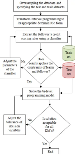
4. Model solving
Fig. 1 shows the overall steps of the decision making process. This paper uses the fuzzy apriori as a classifier in combination with Genetic Algorithm bi-level programming. The following subsections describe the algorithms used.
4.1.Genetic algorithm based bi-level programming algorithm (GABBA)
Genetic algorithm based bi-level programming algorithm is one of the most successful artificial intelligence based methods that have been developed to solve the linear bi-level programming problems (Lee & Shih, 2000). In this algorithm, the leader’s decision vector is reproduced according to the modifications of genetic algorithm and the follower’s decision vector is obtained by solving the lower level linear problem (Lee & Shih, 2000). The process is repeated until achieving the appropriate fitness.
4.2.Fuzzy apriori (FA)
Fuzzy apriori is one of the extensions of traditional apriori algorithm, which is mainly introduced to extract association rules. Fuzzy aproiri can be used for extracting rules and better classification result from fuzzy apriori could be achieved if support and confidence parameters are adjusted. In this paper, an extension to the method proposed by Hu et al. (2003) is used. Genetic algorithm method is replaced with the particle swarm because of its better convergence and ability to reach the better results is less time. This study uses particle swarm to find two parameters of the fuzzy association rules which are fuzzy support (FS) and fuzzy confidence (FC). In addition, a multi objective fitness function is used; Sadatrasoul et al. (2015) used this method and reported its superiority compared with genetic algorithm.
4.3.Combination of GABBA and FA algorithms
The objective functions for financial institutes are convex and the solution space is discrete. Therefore, traditional methods for solving the bi-level programming cannot be used to solve the problem. Bi-level Genetic FA Algorithm (BGFAA) is a combination of traditional bi-level genetic algorithm with fuzzy apriori classification algorithm (Bard, 1998). In this paper, a type of fuzzy apriori rules set is used for the classification (Hu et al., 2003). The fuzzy apriori rules are built using training dataset. The learning process is continued until the stopping criteria met. The experiments are accomplished and the results are reported using the test dataset.
There is an important point about producing and reproducing the decision vectors in BGFAA. It is obvious that decision vector (Xtg,Xa) for the leader and the follower cannot be initialized by
themselves because they are the output of the classification process. In order to handle the issue, the
jth initial point with an ordered pair of (FSj, FCj) is considered, it solves the fuzzy apriori classifier
and a vector of Xa in which ={0,1} can be achieved. Each applicant is active in a special industry
sector and province; therefore the amount of allocated credit can be computed using the credit
dataset. Finally, the amount of allocated credit for each industry sector/province ( ) can be
obtained adding the sum of credit amounts for which =1, and the Xtg vector is being extracted
then. In fact ∀ ∈ → ∑ and Fig. 2 shows the steps of
producing/reproducing the decision vector.
(fsj, fcj) Xaj Xtgj
Extracting jth rule base using fuzzy apriori and computing Xaj
Computing Xtgj using the credit database and Xaj vector values
Fig. 2. Stages of producing/reproducing the decision vectors for the jth point
The proposed BGFAA is presented using following notation:
1 2
I: set of positive real numbers
U[a,b]: uniform distribution between a and b
xtg(k),xa(k): leader and followers decision vectors at generation k
: ith component of the leader’s decision vector , … ,
: ith component of the follower’s decision vector , … ,
, : jth structure of leader and follower decision vectors
and : ith component of the jth structure of vectors xtg and xa
Pj(k): value of the leader’s objective given for , at the kth generation
∏ : population at generation k: ∏ ,
Step 0. Initialization
Let k=0, ∗(-1)=∞, and set parameters:
(a) N=population size
(b) NP= number of current solutions (i.e. structures) in population ̂ to undergo mutation.
(c) NX= number of leader decision variables (i.e., alleles) to undergo mutation
(d) NR= number of new random solutions created during each iteration.
(e) degree of accuracy required.
Step 1. Set bounds
Set [0,1] as lower and upper bounds for pairs of (fs , fc) for fuzzy support and fuzzy confidence.
Set SCALE =10 , such that SCALE fs , fc .
Step 2. Generate initial population , which contains N vectors , ), j=1,…,N, as
follows:
2.1. Implement fuzzy partitioning; with k=3. Therefore each variable is converted two three
linguistic variables include low, medium and high.
2.2. Generate fuzzy apriori rules;
2.2.1. Generate n initial positions, each position is shown by an order pair (fs , fc) between zero and
one.
2.2.2. Generate frequent fuzzy item sets.
2.2.3. Generate fuzzy rules.
2.2.4. Reduce redundant rules.
2.2.5. Use adaptive rules to adjust fuzzy rule's weights.
2.3. Create decision vectors (Xtg,Xa) for each pair (fs , fc).
2.3.1. If ~ ⋃ , , i=1,…,n exclude the result,
2.3.2. Solve the follower problem (leader and followers constraints included)
(a) If feasible, store rational reaction ; If j=N, go to step 3;
Else put ← 1 and go to step 2.2
Step 3.SCALE modification
Sort array ∏ according to level 1 objective: , 1, … ,
(i.e. , ∀j
Store ∗ and ∗ , ∗ ∗
Let F k ∑ F k
If F∗(k)= F∗(k-1) and if F
. k 0.15 F∗(k), then SCALE =SCALE/10
Step 4.Stopping criteria
If SCALE , then stop; satisfactory soluction is ∗ , ∗ , otherwise go to step 5.
Step 5. Mutate structure
Let z , , j=1,…,NP (Note NP N, and z ⊂ z ). Mutate the NP vectors z as follows
(let j=0):
5.1.j=j+1
Obtain = int ((fs , fc /SCALE SCALE ω where ω ∈∪ 0, SCALE .
5.2. Solve the follower problem with leader and followers constraints together
5.2.1. If solution is feasible, store ;
If j=NP, go to step 6 ; else go to step 5.1.
5.2.2. If solution is infeasible, discard and go to step 5.1.
Step 6. Random structure
Let z =( , 1, … , .
Generate NR vectors z as follows (let j=0): 6.1.j=j+1 ~ ⋃ , , 1, … ,
6.2. Solve the follower problem with leader and followers constraints together
6.2.1. If feasible, store .
If j=NR, go to step 7; else go to step 6.1.
6.2.2. If feasible, discard and go to step 6.1.
Step 7. Selection
From the N x , structures from ∏ k , from the NP or less , structures from
mutation, and from the NR , population from random structures, select the N
structures that have smallest values of F(0) to form ∏ k 1 .
Put ← 1 and go to step 3.
5. Experiments, results and discussion
In order to show the model’s applicability, an Iran’s sovereign wealth fund called national development fund (NDF) has been selected as the government related institutes as the leader and one of its agent banks is selected as the follower. NDF allocate its investment in a risk adjusted portfolio of loans and other investments. There are few published works in the literature for SWFs. Yu et al. (2010) introduced a maximum CRRA utility and minimum VAR objective to optimize strategic assets allocation of SWFs. They used NSGA-II to achieve the Pareto solutions. This paper has used a mathematical model in order to model credit allocation in NDF. This section contains three sub sections, in the first one the used data sets are described, the second subsection describes the experiments designs and finally in the third subsection the results and discussions are described.
5.1The data sets
Data availability restrictions have forced the study to use one of the NDF’s agent banks dataset in order to evaluate the performance of the proposed method. The initial dataset included 1109 corporate applicants and 60 financial and non-financial variables in the period from 2009 to 2012. First, a data cleaning process has been performed on the data, including removing redundant, outlier's data and missing values. There were a few missing values for some corporate, some of them did not have financial data and the others did not have the result of their loans; in fact, they were in the process of debt repay. Therefore, 387 corporates were excluded. Out of 722 remaining corporates, 652 companies were credit worthy and other 70th were unworthy. Once the data cleaning process was completed, the categorical variables including the type of industry; type of company and the book type were converted to numerical variables using dummy variables. The results and descriptions of the changes are shown in appendix (1). Using dummy variables number of variables has increased to 60. The main dataset had nearly a 90/10 class distribution. To avoid over fitting, the G/B odd's ratio of 3:1, which was proposed in other major credit scoring studies has been used in this paper (Chi & Hsu, 2011; Chuang & Chen, 2006). Besides, since over-sampling generally gives better performance than under sampling, random minority over sampling (ROS) has been used to over sample the applicants labeled as Bad. Finally, the numbers of data, the numbers of good and bad numbers are reported in Table 1.
Table 1
Credit dataset description
Status Data Size Good / All (%) Total Continuous Inputs Features Categorical
Before cleaning 1109 NA 51 43 8
After cleaning 722 90.3 60 39 21
Balanced dataset 869 75.02 60 39 21
There are four types of industries examined in the models including agriculture, service, oil/petrochemical and industry/mine sector. The data for Balassa index and computations have been adopted from the world trade organizations statistics year book (World Trade Organization, 2012). Location quotient data were taken from international labor organization and OECD statistics (OECD, 2012). Direct, indirect and induced job creation in each industrial sector per 1 million dollars of investment were provided from political economy research institute reports (Heintz, et al., 2009). Because the leader and the follower have multiple objective functions, the global criterion method with p =1 has been used in order to convert the multi objective problem into a single objective problem. In order to simplify the computations, BGFAA is run for 3 provinces and 2 industry sectors.
The parameters for BGFAA were defined as 10, 2, 1, 3, C 30 and the
last runs were performed using the tuned for lower and upper parameters of objective functions and constraints as shown in Table 2.
Table 2
Upper and lower limits for different parameters of numerical example
Parameter name Lower limit Upper limit Parameter name Lower limit Upper limit
C 3,000 3,000 Cg ∀ 600 1,500 EBa ∀ 1.7 5 Ct ∀ 650 2,000 EB 2 5 Ee 20,000 50,000 MRa ∀ 0 3.8 Ege ∀ 0.001 0.01 MR 0 3.2 Ete ∀ 1,500 10,000 CAWAg∀ 300 - Ei 10,000 35,000 CAWA 1000 - Egi ∀ 0 0.01 CCT 10,000 30,000 Eti ∀ 8,000 20,000 AIM 0.4 1
5.2Experiments design
Two different scenarios have been built in order to evaluate the credit allocation strategy. One of the designed scenarios uses the bi-level programming with classification and the other one uses a simple multi objective problem. These scenarios are briefly described as follows:
Scenario (I): NDF as the leader and Agent banks as the follower: In this scenario, NDF is the
leader and the agent bank is follower. the problem is solved using BGFAA,
Scenario (II): NDF as the dominant policy maker: In this scenario, NDF decides on the
industrial sectors/province credit allocation variables Xtg. Although this scenario may not be
feasible in a real environment.
5.3Results and Discussion
Table 3 shows different objective function values for scenarios of the study. The minimum NDF risk is bolded. For other maximization objectives including return, competitive advantage, local economy, current account and experience with bank the best results are also bolded.
Table 3
Different objective functions values for different scenarios
NDF Agent bank
Scenario NO. Return Risk Competitive advantage Local economy Current account Experience with bank
(I) 0.0117 0.00018 0.34636 0.54974 99.8 12.782
(II) 0.03215 0.00193 0.237466 0.607 -
-According to the results of Table 3, for the NDF return and risk, the second scenario is ranked first followed by the first scenario. For the competitive advantage objective, the first scenario is better and finally for the local economy, the second scenario is better. It is obvious that the objective functions for the second scenario can be better as they are not subjected to agent banks’ objectives and constraints. There is another important issue and that is the agent bank cannot collaborate with NDF in credit allocation process as the imposed credit allocation scenario by NDF cannot pass its minimum requirements, which are modeled by its constraints. Therefore, although the first scenario gives less valuable results but according to modeling the problem in a bi-level programming it is the only scenario that can work. Another important issue is that depending on the parameters of the leader and follower, a special problem may not have any answer. In that situation, the second scenario would have answer also.
6. Conclusion
Credit allocation is a critical issue for both public and private sectors in the economy. In situations where collaboration is inevitable, it is of double complexity because each partner has its own preferences modeled in terms of objectives and constraints are in conflict with each other. This paper has introduced a new leadership-followership strategy and used Stackelberg game to mathematically model the situation. The game has been modeled using a bi-level programming problem in which the first level used the profitability and sustainable development concepts and the second level used credit scoring and profit scoring. The approach has been applied for a national development fund (NDF) and one of its agent banks. Two different scenarios have been explained. In order to solve the game, a new algorithm named Bi-level Genetic FA Algorithm (BGFAA) has been introduced. This algorithm used a type of fuzzy apriori as a classification algorithm in the heart of bi-level genetic algorithm to solve the designed game. The mentioned bilateral scenario has been experimented against a unilateral scenario in which the NDF was the dominant policy maker. The results have indicated that by including the role of agent bank, competitive advantage and agent banks objectives were in their best situation. The potential future work in the area could be considered on other applications of the algorithm in the areas of credit allocation can be also practiced.
References
Bard, J. F. (1998). Practical bilevel optimization: algorithms and applications: Springer.
Bard, J. F., Plummer, J., & Claude Sourie, J. (2000). A bilevel programming approach to determining tax credits for biofuel production. European Journal of Operational Research, 120(1), 30-46.
Chi, B. W., & Hsu, C. C. (2012). A hybrid approach to integrate genetic algorithm into dual scoring
model in enhancing the performance of credit scoring model. Expert Systems with
Applications, 39(3), 2650-2661.
Chuang, R. J., & Chen, M. J. (2006). The building of credit scoring system on the residential mortgage finance.
International Journal of Forecasting, 15(2), 65–90.
Colson, B., Marcotte, P., & Savard, G. (2005). Bilevel programming: A survey. 4OR: A Quarterly Journal of
Operations Research, 3(2), 87-107.
De Benedictis, L., & Tamberi, M. (2001). A note on the Balassa index of revealed comparative advantage.
Available at SSRN 289602.
Desai, V. S., Conway, D. G., Crook, J. N., & Overstreet, G. A. (1997). Credit-scoring models in the
credit-union environment using neural networks and genetic algorithms. IMA Journal of
Management Mathematics, 8(4), 323-346.
Economic, U. N. D. o. (2007). Indicators of sustainable development: Guidelines and methodologies: United
Nations Publications.
Finlay, S. (2010). Credit scoring for profitability objectives. European Journal of Operational Research, 202(2), 528-537.
Finlay, S. (2011). Multiple classifier architectures and their application to credit risk assessment. European
Journal of Operational Research, 210(2), 368-378.
Firth, M., Lin, C., Liu, P., & Wong, S. M. L. (2009). Inside the black box: Bank credit allocation in China’s private sector. Journal of Banking & Finance, 33(6), 1144-1155.
Gholamian, M. R., Sadatrasoul, S., & Hajimohammadi, Z. (2012). Fuzzy Apriori Rule Extraction Using Multi-Objective Particle Swarm Optimization: The Case of Credit Scoring. Journal of Advances in Computer
Research, 3(3), 53-64.
Harrell, F. E., & Lee, K. L. (1985). A comparison of the discrimination of discriminant analysis and logistic regression under multivariate normality. Biostatistics: Statistics in Biomedical; Public Health; and
Environmental Sciences. The Bernard G. Greenberg Volume. New York: North-Holland, 333–343.
Harrell, F. E., & Lee, K. L. (1985). A comparison of the discrimination of discriminant analysis and logistic regression under multivariate normality. Biostatistics: Statistics in Biomedical, Public Health and
Environmental Sciences’, North-Holland, New York, United States, 333-343.
Heintz, J., Pollin, R., & Garrett-Peltier, H. (2009). How infrastructure investments support the US economy: employment, productivity and growth. Political Economy Research Institute (PERI), University of
Massachussetts Amberst.
Hu, Y.-C., Chen, R.-S., & Tzeng, G.-H. (2003). Finding fuzzy classification rules using data mining techniques. Pattern Recognition Letters, 24(1), 509-519.
Hu, Y. C., Chen, R. S., & Tzeng, G. H. (2003). Finding fuzzy classification rules using data mining techniques.
Pattern Recognition Letters, 24(1-3), 509-519.
Huang, C. L., Chen, M. C., & Wang, C. J. (2007). Credit scoring with a data mining approach based on support vector machines. Expert Systems with Applications, 33(4), 847-856.
Hunt, S. D., & Morgan, R. M. (1995). The comparative advantage theory of competition. The Journal of
Marketing, 59(2), 1-15.
Lahsasna, A., Ainon, R. N., & Wah, T. Y. (2010). Credit scoring models using soft computing methods: A Survey. International Arab Journal of Information Technology, 7(2), 115-123.
Laursen, K. (1998). Revealed comparative advantage and the alternatives as measures of international specialisation. DRUID Working Papers.
Lee, E. S., & Shih, H.-S. (2000). Fuzzy and Multi-Level Decision Making: And Interactive Computational
Approach: Springer-Verlag New York, Inc.
Lee, Y. C. (2007). Application of support vector machines to corporate credit rating prediction. Expert Systems
with Applications, 33(1), 67-74.
Leite, S. P., & Vaez-Zadeh, R. (1986). Credit allocation and investment decisions: The case of the manufacturing sector in Korea. World Development, 14(1), 115-126.
Meisel, S., & Mattfeld, D. (2010). Synergies of operations research and data mining. European Journal of
Operational Research, 206(1), 1-10.
OECD. (2012). OECD Main Economic Indicators Retrieved from http://www.imd.ch/wcy
Ryu, J.-H., Dua, V., & Pistikopoulos, E. N. (2004). A bilevel programming framework for enterprise-wide process networks under uncertainty. Computers & Chemical Engineering, 28(6), 1121-1129.
Sadatrasoul, S., Gholamian, M., & Shahanaghi, K. (2015). Combination of Feature Selection and Optimized Fuzzy Apriori Rules: The Case of Credit Scoring. The International Arab Journal of Information
Technology 12(2).
SCI, s. c. o. I. (2011). Iran’s statistical yearbook 2013.
Sengupta, A., Pal, T. K., & Chakraborty, D. (2001). Interpretation of inequality constraints involving interval coefficients and a solution to interval linear programming. Fuzzy Sets and Systems, 119(1), 129-138.
Streimikiene, D., Ciegis, R., & Grundey, D. (2007). Energy indicators for sustainable development in Baltic States. Renewable and Sustainable Energy Reviews, 11(5), 877-893.
Thomas, L. C. (2000). A survey of credit and behavioural scoring: forecasting financial risk of lending to consumers. International Journal of Forecasting, 16(2), 149-172.
Thomas, L. C., Edelman, D. B., & Crook, J. N. (2002). Credit scoring and its applications: Siam.
Utkulu, U., & Seymen, D. (2004). Revealed Comparative Advantage and Competitiveness: Evidence for
Turkey vis-à-vis the EU/15. Paper presented at the European Trade Study Group 6th Annual Conference,
ETSG, Nottingham.
von Stackelberg, H. (1952). The Theory of Market Economy: Translated from the German and with an Introd.
by Alan T. Peacock: W. Hodge.
World Trade Organization, W. (2012). International Trade Statistics 2012 Retrieved from
http://www.wto.org/english/res_e/statis_e/its2012_e/its2012_e.pdf
Xiuli, Z., Lianjun, L., & Yunkui, X. (2012). Banking system reform, earnings quality and credit allocation.
China Journal of Accounting Research, 5(3), 217-229.
Yu, J., Xu, B., Yang, H., & Shi, Y. (2010). The strategic asset allocation optimization model of sovereign wealth funds based on maximum CRRA utility & minimum VAR. Procedia Computer Science, 1(1),
2433-2440. Appendix 1
Variables included in credit dataset, and their types are sorted alphabetically and shown in Table 3.
Table 4
List of variables in commercial bank credit dataset
Type Variable Type Variable Continuous Prior period shareholder Equity
Continuous Accounts receivable
Continuous Sale
Continuous Accumulated gains or losses
Categorical seasonal factors
Categorical Active in internal market
Continuous shareholder Equity
Categorical Audit report
Continuous Short-term financial liabilities
Continuous Average exports over the past three years
Continuous Stock
Continuous Capital
Continuous Target market risk (from 1 to 5)
Continuous Company background (number of years)
Continuous Tehran stock exchange index
Continuous Current Account Weighted Average
Continuous three prior year foreign exchange rate
Continuous Current accounts creditor turn over
Categorical Top Mangers history
Continuous Current assets Continuous Total assets Continuous Current liabilities Continuous Total liabilities Continuous Current period assets
Continuous Two-Prior period assets
Continuous Current period sales
Continuous Two-Prior period sales
Continuous Current period shareholder Equity
Continuous Two-Prior period shareholder Equity
Continuous Experience with Bank(number of years in 5 categories)
Categorical Type of book: Accredited auditor (=1,other=0)
Continuous Export price index
Categorical Type of book: Audit Organization (=1,other=0)
Continuous Financial costs
Categorical Type of book: Tax declaration(=1,other=0)
Continuous Gross profit
Categorical Type of company: Cooperative (=1, other =0)
Continuous Inflation rate
Categorical Type of company: Limited and others (=1, other =0)
Continuous Inventory cash
Categorical Type of company: PJS (=1, other =0)
Continuous Last three years average imports
Categorical Type of company: Stock Exchange (=1, other =0)
Continuous Long-term financial liabilities
Categorical Type of company: Stock Exchange(LLP) (=1, other =0)
Continuous Mangers history
Categorical Type of industry: agricultural (=1, other =0)
Continuous Net profit
Categorical Type of industry: chemical (=1, other =0)
Continuous Non-current assets
Categorical Type of industry: industry and mine (=1, other =0)
Continuous Non-current liabilities
Categorical Type of industry: infrastructure and service(=1, other =0)
Continuous number of countries that the company export to
Categorical Type of industry: oil and petrochemical(=1, other =0)
Continuous Other Accounts receivable
Categorical year of financial ratio
Continuous Prior period assets
Categorical )
0 = other,1=) Creditworthy :lebasBy Continuous