2018
Explanatory and Causality Analysis in Software Engineering
Explanatory and Causality Analysis in Software Engineering
Yasser Ali Alshehri [email protected]
Follow this and additional works at: https://researchrepository.wvu.edu/etd Part of the Computer Engineering Commons
Recommended Citation Recommended Citation
Alshehri, Yasser Ali, "Explanatory and Causality Analysis in Software Engineering" (2018). Graduate Theses, Dissertations, and Problem Reports. 3688.
https://researchrepository.wvu.edu/etd/3688
This Dissertation is protected by copyright and/or related rights. It has been brought to you by the The Research Repository @ WVU with permission from the rights-holder(s). You are free to use this Dissertation in any way that is permitted by the copyright and related rights legislation that applies to your use. For other uses you must obtain permission from the rights-holder(s) directly, unless additional rights are indicated by a Creative Commons license in the record and/ or on the work itself. This Dissertation has been accepted for inclusion in WVU Graduate Theses, Dissertations, and Problem Reports collection by an authorized administrator of The Research Repository @ WVU.
Software Engineering
Yasser Ali Alshehri
Dissertation submitted to the
Benjamin M. Statler College of Engineering and Mineral Resources at West Virginia University
in partial fulfillment of the requirements for the degree of
Doctor of Philosophy in
Computer Engineering
Katerina Goseva-Popstojanova, Ph.D., Chair Hany H. Ammar, Ph.D.
Gianfranco Doretto, Ph.D. Vinod Kulathumani, Ph.D. Mario Perhinschi, Ph.D.
Lane Department of Computer Science and Electrical Engineering
Morgantown, West Virginia 2018
Keywords: Software fault proneness, software development effort, explanatory model, case-control study, conditional logistic regression, ordinal logistic regression, causality
regression, structural equation modelling
Explanatory and Causality Analysis in Software Engineering
Yasser Ali Alshehri
Software fault proneness and software development efforts are two key areas of software engineering. Improving them will significantly reduce the cost and promote good planning and practice in developing and managing software projects. Traditionally, studies of software fault proneness and software development efforts were focused on analysis and prediction, which can help to answer questions like ‘when’ and ‘where’. The focus of this dissertation is on explanatory and causality studies that address questions like ‘why’ and ‘how’.
First, we applied a case-control study to explain software fault proneness. We found that Bugfixes (Prerelease bugs), Developers, Code Churn, and Age of a file are the main contributors to the Postrelease bugs in some of the open-source projects. In terms of the interactions, we found that Bugfixes and Developers reduced the risk of post release software faults. The explanatory models were tested for prediction and their performance was either comparable or better than the top-performing classifiers used in related studies. Our results indicate that software project practitioners should pay more attention to the prerelease bug fixing process and the number of Developers assigned, as well as their interaction. Also, they need to pay more attention to the new files (less than one year old) which contributed significantly more to Postrelease bugs more than old files.
Second, we built a model that explains and predicts multiple levels of software develop-ment effort and measured the effects of several metrics and their interactions using categorical regression models. The final models for the three data sets used were statistically fit, and performance was comparable to related studies. We found that project size, duration, the ex-istence of any type of faults, the use of first- or second generation of programming languages, and team size significantly increased the software development effort. On the other side, the interactions between duration and defective project, and between duration and team size reduced the software development effort. These results suggest that software practitioners should pay extra attention to the time of the project and the team size assigned for every task because when they increased from a low to a higher level, they significantly increased the software development effort.
Third, a structural equation modeling method was applied for causality analysis of soft-ware fault proneness. The method combined statistical and regression analysis to find the direct and indirect causes for software faults using partial least square path modeling method. We found direct and indirect paths from measurement models that led to software postrelease bugs. Specifically, the highest direct effect came from the change request, while changing the code had a minor impact on software faults. The highest impact of the code change
indirect impact from code characteristics to software fault proneness was higher than the di-rect impact. We found a similar level of didi-rect and indidi-rect impact from code characteristics to code change.
Acknowledgments
I start with the name of God and then my father and my mother, who were always with me sharing joys and watching my growth in this life. I grieve because they are no longer alive to see this special moment. I know how it would have made them feel.
The dissertation could not have been accomplished without the assistance, patience, and support of many individuals. First to be thanked is my great teacher and advisor Prof. Katerina Goseva-Popstojanova, who taught me so many aspects of research and what should strong research looks like. I learned from her immense knowledge how to be a great researcher, reviewer, teacher, and data scientist.
I offer gratitude to my family back home, to my inspiring brother Dr. Mohammed, my sister Hind, and my nieces and nephew. Many thanks are due to my grandmothers, uncles, and aunties for their love and good wishes and to my family in West Virginia, including my wife Aeshah and my little sweetheart Rawan, who was born in the first year of my Ph.D. journey. Special thanks go to my West Virginian family member Noble N. Nkwocha, his wife Karen Anthony, and their children for all their support and love.
I offer special thanks to my supervisor, Mr. Dale Dzielski from the Lane Department of Computer Science and Electrical Engineering (LCSEE). Throughout my work as a graduate service assistant, he always guided me to achieve the best. Many thanks are due to Dr. Brian Woerner, the chair of the LCSEE department, Dr. Muhammad Choudhry, the chair of the Computer Engineering program, and Dr. Bojan Cukic, the chair of the Computer Science department at the University of North Carolina at Charlotte for their support.
I would also like to extend my thanks to Dr. Hany Ammar, Dr. Gianfranco Doretto, and Dr. Vinod K. Kulathumani; I learned a great deal from them through their courses Advanced Real-Time Systems, Machine Learning, and Sensor Networks. Many thanks to them and to Dr. Mario Perhinschi for agreeing to serve on my PhD committee and guiding my research with their valuable comments and suggestions.
My gratitude extends to my friends in the lab who were very supportive. Special thanks go to Thomas Devine for his support and for providing me with the extracted dataset metrics of Eclipse releases. I would like to thank Mohammad J. Ahmad for providing me with the extracted metrics of the Apache projects. Special thanks are also extended to Jary Hernandez and my other fellows in the lab, Thomas Kyanko, Di Pang, and Jacob Tyo.
Contents
Abstract
Acknowledgments iv
List of Figures vii
List of Tables x
1 Introduction 1
2 Related Works 5
2.1 Related Works on Software Fault Proneness . . . 6
2.1.1 Analysis studies on software fault proneness . . . 6
2.1.2 Software fault proneness prediction . . . 7
2.1.3 Explanatory studies on software fault proneness . . . 10
2.2 Explanatory Work on Software Development Efforts . . . 12
2.3 Related Works on Causality . . . 17
3 Using a Case-control Study to Explain Software Fault Proneness 23 3.1 Background and Motivation . . . 24
3.2 Methodology . . . 29
Confounder Selection and Matching . . . 30
3.2.1 Building the Model . . . 32
The initial model . . . 32
Multicollinearity diagnoses . . . 33
Full model . . . 34
3.2.2 Eliminating interactions . . . 34
3.2.3 Eliminating confounders . . . 35
3.2.4 Goodness of Fit Test . . . 38
3.3 Using a Case-control Study on Eclipse . . . 40
3.3.1 Case Study 1: Europa . . . 40
Confounder Selection, Sampling, and Matching . . . 40
Exposure and Confounder Selection . . . 42
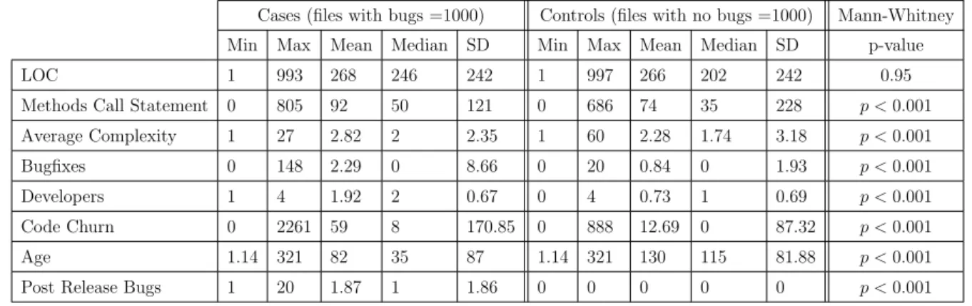
Basic Statistics . . . 44
Building the Model . . . 45
Eliminate confounders . . . 48
Discussion of the results . . . 53
3.3.2 Case Study 2:Ganymede . . . 56
Discussion of the results . . . 59
3.4 Replicated Study: Using a Case-control Study on Apache Projects . . . 63
3.4.1 Derby Project . . . 65
Inclusion and Exclusion . . . 65
Derby 10.1.3.1 . . . 66 Derby 10.4.1.3 . . . 71 Derby 10.5.1.1 . . . 75 Derby 10.6.1.0 . . . 78 Derby 10.8.1.2 . . . 82 Derby 10.8.3.0 . . . 86
Goodness of Fit Test for Derby Models and a Discussion of the Results 88 3.4.2 Ant Project . . . 92
Inclusion and Exclusion . . . 92
Ant 16 . . . 93
Ant 18 . . . 98
Goodness of Fit Test of Ant Models and Discussion of the Results . . 102
3.4.3 Xalan Project . . . 105
Inclusion and Exclusion . . . 105
Xalan 24 . . . 105
Xalan 26 . . . 110
Goodness of Fit Test of Xalan Models and Discussion of the Results . 114 3.5 Discussion of the Results Across All Case Studies: Europa, Ganymede, Ant, Derby, and Xalan . . . 117
3.6 Threats to Validity for Software Faults Proneness . . . 122
3.7 Conclusion for Case-control Study . . . 123
4 Software Fault Proneness Prediction 125 4.1 Introduction and Motivation . . . 126
4.2 Approach . . . 128
4.2.1 Machine learning algorithms . . . 129
4.2.2 Performance metrics . . . 131
4.2.3 Statistical comparisons of results . . . 133
4.3 Datasets and Features Definition . . . 134
4.3.1 Features . . . 134
4.4 Results and Discussion . . . 136
4.5 Threats to Validity for the Software Fault Proneness Prediction . . . 148
4.6 Conclusion for the Software Fault Proneness Prediction . . . 149
5 Explanatory and Prediction Studies of Software Development Effort 150 5.1 Introduction and Motivation . . . 151
5.2 Methodology . . . 155
5.3.1 Data Preprocessing . . . 156
Missing Values . . . 158
Discretization . . . 159
5.3.2 Correlation Test . . . 161
Spearman Correlation Test for Numerical Confounders . . . 161
Level of Association Test for Categorical Metrics . . . 162
5.3.3 Building the Model . . . 163
Multicollinearity Test for the Initial Model . . . 165
Eliminate Interactions . . . 165
Eliminate Metrics . . . 169
Goodness of Fit . . . 169
5.3.4 Explanation of the results . . . 170
Interaction Results . . . 173
5.4 Second Case Study: Desharnais . . . 175
5.5 Third Case Study: Maxwell . . . 184
5.6 Prediction . . . 191
5.6.1 Multi-Class Classification . . . 192
5.6.2 Performance Metrics . . . 194
5.7 Threats to Validity . . . 196
5.8 Conclusion . . . 198
6 The Study of Causality 199 6.1 Motivation and Background . . . 200
6.2 Methodology . . . 204
6.3 Case Study Eclipse’s Europa Release . . . 205
Initial selection of variables . . . 207
Assessing non-normality . . . 207
Sampling . . . 209
6.3.1 Model specification of Europa . . . 211
Measurement models . . . 211
Structural model . . . 217
6.3.2 Model estimation . . . 219
6.3.3 Model validation and goodness of fit . . . 222
6.4 Threats to validity . . . 224
6.5 Conclusion . . . 224
7 Conclusion 226
List of Figures
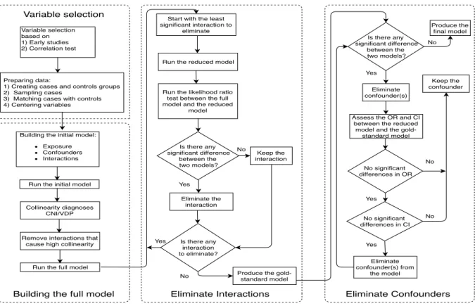
3.1 Flow chart of the methodology for conducting Case-control studies of software
fault proneness . . . 30
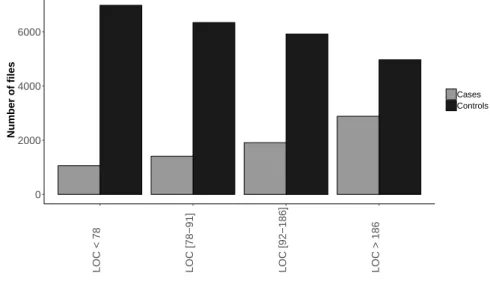
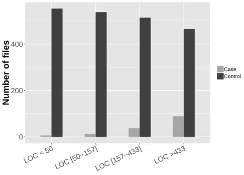
3.2 Distribution of lines of code on cases and controls of Europa . . . 41
3.3 Number of exposed files (Bugfixes=1) in cases and controls . . . 42
3.4 Selected confounders’ boxplots of cases and controls . . . 46
3.5 Europa final model odd ratios and confidence intervals . . . 52
3.6 Significant interaction plots of Europa . . . 55
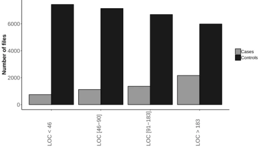
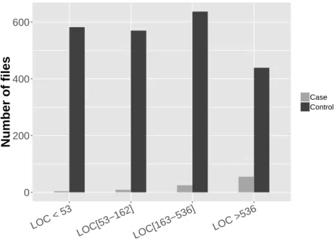
3.7 Distribution of lines of code on cases and controls of Ganymede . . . 57
3.8 Number of exposed files (Bugfixes=1) in cases and controls . . . 57
3.9 Selected confounders’ boxplots of cases and controls in Ganymede . . . 58
3.10 Ganymede final model odd ratios and confidence intervals . . . 61
3.11 Significant interactions of Ganymede releases . . . 63
3.12 The number of faulty files and fault-free files in every release of Derby . . . . 66
3.13 Number of files exposed to Bugfixes from cases and controls for every release of Derby . . . 66
3.14 Distribution of lines of code in cases and controls of Derby.10.1.3.1 . . . 67
3.15 The pair-wise correlation test on Derby 10.1.3.1 using the Spearman correla-tion . . . 68
3.16 The distribution of lines of code in the case and control groups of Derby 10.4.1.3 72 3.17 The pair-wise correlation test on Derby 10.4.1.3 using the Spearman test. . 72
3.18 The distribution of the lines of code in the case and control groups of Derby 10.5.1.1 . . . 76
3.19 The pair-wise correlation test on Derby 10.5.1.1 using the Spearman test . . 77
3.20 The distribution of the lines of code in the case and control groups Derby 10.6.1.0 . . . 79
3.21 The pair-wise correlation test on Derby 10.6.1.0 using the Spearman correlation 80 3.22 The distribution of lines of code in the case and control groups of Derby 10.8.1.2. 83 3.23 A pair-wise correlation test on Derby 10.8.1.2 using the Spearman correlation. 84 3.24 The distribution of lines of code in the case and control groups of Derby 10.8.3.0. 86 3.25 A pair-wise correlation test on Derby 10.8.3.0 using the Spearman correlation 87 3.26 Significant interactions of Derby releases. . . 91
3.27 The final OR of models for Derby releases . . . 92
3.28 The distribution of faulty and fault-free files in the Ant releases . . . 93
3.30 Distribution of the Lines of code confounder in cases and controls in Ant16 . 94
3.31 A pair-wise correlation test on Ant 16 using the Spearman correlation . . . 95
3.32 The distribution of the Lines of code confounder in the case and control groups in Ant18 . . . 99
3.33 A pair-wise correlation test on Ant18 using the Spearman correlation . . . . 100
3.34 Significant interactions in Ant releases . . . 104
3.35 The final results for Ant releases . . . 104
3.36 The number of faulty files and fault-free files in every release of Xalan . . . . 106
3.37 The number of faulty files and fault-free files in the case and control groups in every release of Xalan . . . 106
3.38 The distribution of the Lines of code confounder in the case and control groups in Xalan24 . . . 107
3.39 A pair-wise correlation test on Xalan24 using the Spearman correlation . . . 108
3.40 The distribution of Lines of code in the case and control groups in Xalan26 . 111 3.41 A pair-wise correlation test on Xalan26 using the Spearman correlation. . . . 112
3.42 Interactions from the Xalan24 release . . . 116
3.43 The final results for the Xalan releases . . . 117
4.1 Prediction of fault proneness approach repeated 100 times, on random samples 132 4.2 Performance metrics of all datasets . . . 137
4.3 Critical difference diagrams . . . 138
4.4 Performance metrics for Europa . . . 139
4.5 Performance metrics for Ganymede . . . 140
4.6 Performance metrics for Derby project . . . 141
4.7 Performance metrics for Ant project . . . 142
4.8 Performance metrics for Xalan project . . . 143
5.1 Summary of the methodology of this research . . . 157
5.2 Basic statistics graphs of selected metrics of ISBSG data set . . . 160
5.3 Final ORs for the main metrics and interactions of ISBSG . . . 173
5.4 ISBSG significant interactions . . . 174
5.5 Basic statistics graphs of selected metrics of the Desharnais data set . . . 177
5.6 Final ORs for the main metrics and interactions of Desharnais . . . 182
5.7 Desharnais: Manager experience and project size interaction . . . 183
5.8 Basic statistics graphs of selected metrics in the Maxwell data set . . . 186
5.9 ORs for the main metrics and interactions for the Maxwell data set . . . 190
5.10 Maxwell: Staff availability and efficiency requirements interaction . . . 191
5.11 Processes for prediction . . . 192
5.12 Recall precision and F-score of Effort levels of ISBSG, Desharnais, and Maxwell . . . 193
5.13 MMRE, MdMRE, and PRED(25) for average points and median points of estimate for the three data sets . . . 196
6.1 Methodology of the causality research . . . 206
6.3 Distribution of the initial independent variables . . . 210 6.4 Measurement model . . . 213 6.5 Change request and change code latent variables correlation test results . . . 215 6.6 Structural model . . . 219
List of Tables
3.1 CNI/VDP collinearity diagnoses for Europa Model0 . . . 34
3.2 Odd ratios test for eliminating confounders . . . 38
3.3 Confidence intervals test for eliminating confounders . . . 38
3.4 Static code and change confounders used in this study . . . 43
3.5 Spearman correlation coefficients for Europa release . . . 44
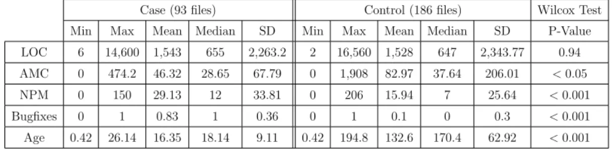
3.6 Basic statistics for cases and controls samples of Europa . . . 45
3.7 CNI/VDP collinearity diagnoses for Europa’s initial model Model0 . . . 49
3.8 Europa release model reduction using backward hierarchal elimination for interactions . . . 50
3.9 The eight scenarios to consider in eliminating the confounders . . . 51
3.10 Golden standard odds ratio and odds ratios of scenario 8 . . . 51
3.11 Confidence interval assessment of Europa . . . 51
3.12 Basic statistics for cases and controls samples of Ganymede . . . 57
3.13 Spearman correlation coefficients for the Ganymede release . . . 58
3.14 Ganymede release model reduction using backward hierarchal elimination for interactions . . . 60
3.15 Release date of Derby releases . . . 65
3.16 Descriptive data of case and control groups of Derby 10.1.3.1 . . . 67
3.17 The CNI/VDP collinearity diagnosed for model Derby.10.1.3.10 . . . 68
3.18 The Derby.10.1.3.1 release model reduction using backward hierarchal elimi-nation for the interactions . . . 69
3.19 The odds ratio comparison between the Derby.10.1.3.1OR∗ model and the Derby.10.1.3.1OR2 model . . . 70
3.20 Descriptive data of cases and controls of Derby 10.4.1.3 . . . 71
3.21 The CNI/VDP collinearity diagnosed for model Derby.10.4.1.30 . . . 73
3.22 The Derby 10.4.1.3 release model reduction using backward hierarchal elimi-nation for the interactions . . . 73
3.23 Odds ratio comparison between the Derby.10.4.1.3OR∗model and the Derby.10.4.1.3OR2 model . . . 75
3.24 The descriptive data of the case and control groups of Derby 10.5.1.1 . . . . 75
3.25 CNI/VDP collinearity diagnosed for the model Derby.10.5.1.10 . . . 77
3.26 Derby 10.5.1.1 release model reduction using backward hierarchal elimination for the interactions . . . 78
3.28 The CNI/VDP collinearity diagnosed for model Derby.10.6.1.00 . . . 80
3.29 Derby.10.6.1.0 release model reduction using backward hierarchal elimination for the interactions . . . 81
3.30 The OR and CI assessments between Derby.10.6.1.0OR∗ and Derby.10.6.1.0OR2 82 3.31 Descriptive data of cases and controls groups of Derby.10.8.1.2 . . . 83
3.32 The CNI/VDP collinearity diagnosed for model Derby 10.8.1.20 . . . 84
3.33 Derby.10.8.1.2 release model reduction using backward hierarchal elimination for the interactions . . . 85
3.34 The OR and CI assessments between Derby.10.8.1.2OR∗ and Derby.10.8.1.2OR2 86 3.35 The descriptive data of case and control groups of Derby.10.8.3.0 . . . 87
3.36 The CNI/VDP collinearity diagnosed for model Derby.10.8.3.0f ull . . . 88
3.37 Derby.10.8.3.0 release model reduction using backward hierarchal elimination for the interactions . . . 88
3.38 Results of goodness of fit test according to Hosmer Lemoshow . . . 89
3.39 The distribution of the lines of code confounder in the case and control groups in Ant 16 . . . 94
3.40 The CNI/VDP collinearity diagnosed for model Ant16Model0 . . . 96
3.41 Ant16 release model reduction using backward hierarchal elimination for the interactions . . . 96
3.42 The odds ratios comparison between the gold standard model and the first scenario model . . . 98
3.43 Descriptive data of case and control groups for Ant 18 . . . 98
3.44 The CNI/VDP collinearity diagnosed for model Ant18Model0 . . . 100
3.45 Ant18 release model reduction using backward hierarchal elimination for the interactions . . . 101
3.46 The odds ratios and CI assessment between the gold standard model and the model without NPM and AMC in Ant18 . . . 102
3.47 Goodness of fit test for Ant16Modelf inal and Ant16Modelf inal models accord-ing to Hosmer Lemoshow . . . 102
3.48 Descriptive data of the case and control groups in Xalan24 . . . 107
3.49 The CNI/VDP collinearity diagnose for model Xalan240 . . . 109
3.50 The interaction elimination process for Xalan 24 . . . 110
3.51 Descriptive data of case and control groups of Xalan-26 . . . 112
3.52 The CNI/VDP collinearity diagnosed for model Xalan260 . . . 113
3.53 Xalan26 release model reduction using backward hierarchal elimination for the interactions . . . 114
3.54 Results of the goodness of fit test for models Xalan24f inal and Xalan26f inal according to Hosmer Lemoshow . . . 114
3.55 Answers to the research questions RQ1 across all projects . . . 119
3.56 Answers to research question RQ2 across all projects . . . 121
4.1 Confusion matrix . . . 133
4.2 Training and testing samples of the Eclipse and Apache releases . . . 134
4.3 Metrics at file level used as features . . . 135
4.5 Performance of the G-Lasso per project . . . 145
4.6 Performance (precision, recall , accuracy, and AUC) of this study and related studies . . . 146
4.7 Performance (AUC) of related studies applying top-performing classifiers and imbalance treatment . . . 146
4.8 Summary of the research questions . . . 147
5.1 Metrics definitions . . . 158
5.2 Spearman correlation coefficients for numerical metrics . . . 161
5.3 Association levels of nominal and ordinal metrics . . . 162
5.4 Multicollinearity test results of ISBSG data set . . . 166
5.5 Interaction Elimination Process and Final Model Results . . . 168
5.6 Metrics’ definitions in the Desharnais data set [1] . . . 175
5.7 Spearman correlation coefficients of the numerical metrics of the Desharnais data set . . . 176
5.8 Association levels of nominal and ordinal metrics . . . 178
5.9 Multicollinearity test results of the Desharnais data set . . . 179
5.10 Interactions Elimination Process of Desharains data set . . . 180
5.11 ORs and CIs’ assessment of the Desharnais model . . . 181
5.12 Metrics’ definitions in the Maxwell data set . . . 184
5.13 Association levels of nominal and ordinal metrics . . . 185
5.14 Multicollinearity test results of Maxwell data set . . . 187
5.15 Interactions elimination process of the Maxwell data set . . . 188
5.16 OR and CI assessment of the Maxwell model . . . 189
5.17 MMRE, MdMRE, and PRED(25) for this work and related works . . . 195
5.18 Summarized answers to research questions RQ1, RQ2, andRQ3 . . . 196
6.1 Static code and change variables definitions [2] . . . 208
6.2 Outer weights of the independent variables with 2.5% lower L and 97.6% upper U values of the measurement models . . . 216
6.3 Correlation coefficients of latent variables . . . 217
6.4 Variance inflation factor for the structural models . . . 219
6.5 Results of the structural models . . . 221
6.6 Direct and indirect effects, with 2.5% lower and 97.5% upper bootstrap samples221 6.7 Summary of the research questions . . . 223
Chapter 1
Introduction
This dissertation offers four major contributions to two areas of software engineering. The two areas of study are software fault proneness and software development efforts. Most of the related works are focused on analysis and prediction. This area lacks of explanatory and causality studies. This area also lacks systemic modeling techniques that can overcome challenges associated with the nature of the software project data and provide explanatory models to fit the data. The contributions aim to provide an explanatory approach using methods that (1) consider main confounders1 and their interactions results in models that (2) are not affected by multicollinearity, and (3) and are statistically fit for the data. So, models can explain how different confounders and their interactions are affecting both software fault proneness and software development effort. This can help software practitioners to improve their practice in software development and testing, and in estimating the development effort, which can significantly help to improve quality of software products and reduce the extra cost that results from the inaccurate effort estimation or software faults.
1In this dissertation, depending on the specific approach used, we use different terms for independent
The contributions to these two areas include (1) an explanatory approach using a matched case-control method in the software fault proneness area; (2) an explanatory approach using a categorical regression method for modeling confounders and interactions of confounders in the software development efforts area; and (3) use of the structural equation modeling SEM as a causality modeling technique to explain software fault proneness and direct and indirect effects of different metrics on software faults.
The first contribution of this work is to establish a methodology that can build a well-fitting explanatory model to explain the main contributors of software faults from con-founders (i.e., metrics) and interactions of concon-founders. The methodology is based on a case-control study that accounts for exposure and matching between files in terms of their size. Matching between files can potentially tighten the range of the upper and lower values around the odds (i.e., the probability of success over the probability of failure). We tested conditional logistic regression (CLR) algorithm to allow for matching between files based on their size when the model was built. Further, interactions in the model gave more insight and new explanations that have not been discussed in similar works [3, 4, 5, 6, 7, 8, 9]. The selection of the initial set of confounders was based on the pair-wise correlation coefficients between all pairs of confounders. We divided the data based on the postrelease bugs sta-tus: (1) cases groups are files with one postrelease bug or more and (2) controls group are files with no postrelease bugs. Then, sampling was made for the cases group, followed by matching with files with the same size from the controls group. Then, the initial model was tested for multicollinearity. Lastly, the backward elimination modeling was applied because of the existence of interactions between confounders. The final model was measured for the goodness of fit. We built a total of twelve models from twelve releases of Eclipse and Apache projects. All final models were fit to the data and reported some consistent results across all projects as discussed in more details in Chapter 3.
Second, we measured the prediction performance of the models built for explanatory purposes. We used the same samples and the same models with their confounders and interactions for this purpose. To evaluate the performance of the conditional logistic regres-sion (CLR), we needed to compare the performance with other commonly used classifiers as benchmark. However, for the other classifiers, we were not able to use the interactions of
the confounders. Therefore, we used all the set of the change metrics for all other classifiers. We also applied a new algorithm that accounts for confounders selection and shrinkage by minimizing insignificant confounders’ coefficients to zeros and relied on the remaining met-rics for prediction. This process can automate the manual selection of confounders that was applied earlier and provide good predictions. The prediction performance of this algorithm was compared with the performance of five top-performing classifiers in the area (i.e., logistic regression, naive Bayes, decision tree J48, random forest, and decision list PART). The work of this part is covered in detail in Chapter 4.
Third, we applied an explanatory study in the area of software development effort. This area also lacks systemic modeling techniques that can overcome challenges associated with the nature of the software project data and provide explanatory models to fit the data. Software development effort, measured in man-hours, was discretized to ordinal format with other selected independent confounders. The independent confounders were chosen based on the early findings and popularity of the confounders in the related works. Other considera-tions were made to treat missing data, study the association between independent metrics, and test models for multicollinearity during the process of building the final models. Insignif-icant interactions and metrics were eliminated to leave the model with only signifInsignif-icant terms (i.e., confounders and their interactions). The final models were tested for goodness of fit and the ability of the final models to predict different classes for software development effort were also considered using the most popular performance metrics. The findings regarding the main confounders and interactions can be used by the software project managers and practitioners to help to produce software products with less challenge concerning develop-ment effort. The proposed methodology was applied to three open and private data sets, which discussed in more detail in Chapter 5.
Last, we explored applying the causality concept in the software fault proneness area. Causality is important because there is a clear distinction between correlation and causation. We conducted a causality using one of the popular methods, structural equation modeling (SEM) [10, 11]. We built our own methodology based on several aspects from earlier works. The methodology leads to a final graphical causal model, which includes significant
con-founders and underlying variables (i.e., latent variables) that cause the postrelease faults. The final model was achieved after statistical analysis, model specification, estimation, and model validation. The methodology of this work and the case study using the Eclipse project are explained in Chapter 6.
The rest of this dissertation is organized as follows. A highlight on related studies from all the areas, which includes (1) explanatory and prediction of software fault proneness, (2) explanatory and prediction of software development effort, and (3) causality studies are discussed in Chapter 2. In Chapter 3 we discuss the motivation, methodology, case studies, and results of explanatory work proposed by this study using a case-control method. The prediction of explanatory models and the comparison of prediction performance with other classifiers including the Group Lasso regression algorithm are explained in Chapter 4. The explanatory and prediction studies for the software development effort are discussed in Chapter 5, including the methodology and the case study of the three open and private projects datasets. The causality study of the software fault proneness area is described in Chapter 6. The threats to validity and future directions of research are discussed at the end of each chapter. Last, the dissertation is concluded in Chapter 7.
Chapter 2
Related Works
This chapter highlights related studies of the two areas: software fault proneness and soft-ware development efforts. The chapter focuses on studies that used explanatory approaches in the two areas. Further, it highlights some of the recent studies that applied different approaches of predictions, including the performance they achieve from applying prediction. Additionally, the chapter covers related studies that used the causality approach in software engineering and in other fields. This chapter is organized as follows. The related works on software fault proneness are discussed in Section 2.1. Then, the related works of explanatory and prediction in software development efforts are discussed in Section 2.2. Last, the related works of causality in software engineering and in other fields are explained in Section 2.3. At the end of every section, we describe the novelty our work is adding to the specific area.
2.1
Related Works on Software Fault Proneness
The studies focused on software fault proneness can be classified into three main cate-gories: 1) studies focused on analysis [12, 13, 14, 15, 16, 17, 18, 19]; 2) studies focused on prediction [20, 21, 22, 23, 24, 25, 26, 27, 28, 29, 30, 31]; and 3) studies focused on explanatory methods to identify impacts of metrics on the software fault proneness [3, 4, 5, 6, 7, 8, 9].
2.1.1
Analysis studies on software fault proneness
The first category is based on statistical and quantitative analysis to find relations be-tween different metrics and software faults [12, 13, 14, 15, 16, 17, 18, 19, 32, 33]. Three studies found that LOC are not associated with Postrelease bugs [12, 13, 14]. Other studies found that LOC is negatively correlated with fault density [32, 33]. Fenton and Ohlesson [12] did not find any relation between prerelease and Postrelease bugs using a dataset from Ericsson Telecom. The study found that 72% to 94% of prerelease faults were detected in files with no Postrelease faults. On a contrary, the two replicated studies [13, 14] found the Prerelease bugs and Postrelease bugs are associated. The study [16] found that prerelease and Postrelease faults are positively correlated. Other studies [17, 19] investigated where faults are localized and a common source of failure. Two studies [30, 31] found that 75% of software faults were localized in 20% of files. Misirli et al. [18] used the Spearman test to explain the correlation between change metrics and faults of Eclipse 2.1 and 3.0. The study found a high correlation between age (old files) and Prerelease faults. Additionally, the study found a high correlation between number of revisions and the Postrelease faults. A high correlation was found between the number of developers and Postrelease faults. An-other statistical test (Mann Whitney-U) was used to examine the differences between two groups of files (failure prone, and non failure prone) [15]. Code churn and complexity of the code metrics were found to be statistically significantly different between the two groups. The two metrics were highly associated with software faults on the Eclipse dataset and had a low association in Microsoft Windows Vista. Other metrics were consistent in both systems.
2.1.2
Software fault proneness prediction
The second category of related works dealt with predicting software fault proneness [20, 21, 22, 23, 24, 25, 26, 27, 28, 29, 30, 31]. Predictions were made using mainly two types of modeling: numerical prediction or classification. Models used regression results in numerical values for number of faults in a software unit. At the same time, the output from classification models can tell us if the software unit is faulty or fault free.
Hall et al. [34] reviewed 208 papers in software fault proneness and investigated the algorithms applied, metrics applied, and datasets used. In terms of the algorithms, LR algorithm was used most often (in 40% of papers), followed by the NB algorithm, used in 25%. Other algorithms such as J48, neural networks, and RF were each used by around 8% of papers [34]. Object-oriented metrics were used in 20%, followed by the static code metrics used in 18%. Change metrics, a combination of static code (8%) and change metrics (8%), LOC (8%), and source code (5%), came next. Regarding datasets, 50% of papers used the Eclipse project, 13% used telecom project(s), 12% used Mozilla, and only 1% of papers used Apache projects.
Analysis of specific metrics and their role in improving prediction performance was con-ducted by [28, 29, 25, 35, 36]. Older files (more than a year in age) had fewer faults than new files [28]. Another study [35] found that the number of developers has no impact on software faults. Ostrand et al. [36] developed a prediction model that considered the developers metric to find a number of faults related to every developer. Another two studies found that using the summation of added lines and deleted lines as a code churn metric improved prediction performance [29, 25].
Schr¨oter et al. [20] encouraged to work in mining static metrics, change metrics, and human-related metrics and used them to predict software faults. Zimmermann et al.[23] built classification models for Eclipse releases 2.0, 2.1, and 3.0 and reported precision, recall, and accuracy of all classification models using both file and package levels. The reported accuracy was between 80% and 90%. At the file level, the recall values were very low, not exceeding 30%, and the precision values were between 47% and 72% at the package level. Catal et al. [37] investigated the effects of dataset size, metrics set, and feature selection
techniques on software fault predictions, using NASA datasets from the PROMISE repository and applying nine machine learning algorithms (e.g., J48, RF, NB). In terms of the AUC, RF outperformed other classifiers when used with large datasets, and NB performed the highest when used with small datasets.
Moser et al. [21] investigated whether change metrics provide better prediction than static code metrics. The authors applied several machine learning algorithms to Eclipse releases 2.0, 2.1, and 3.0 and found the change metrics provided better performance than static code metrics on all datasets for all algorithms. Krishnan et al. [22] used change metrics, the same Eclipse releases as [21] and another four releases (Europa, Ganymede, Helios, and Galileo). The predictions were done at file level using the J48 algorithm. In a follow-up work, Krishnan et al. [38] investigated whether the predictions of software fault proneness improved as the Eclipse product line evolved. The study found that there was no statistically significant difference between the AUC and the true positive rate (TPR) of the top algorithms, including J48. Therefore, J48 was used, and its performance on releases 2.0, 2.1, and 3.0 was compared with the previous works [23, 21].
Gue et al. [39] analyzed the performance of RF with other machine learning algorithms (e.g., logistic regression, J48, Naive Bayes, and random forest). The study used five datasets from NASA project, applied different types of features (e.g., McCabe complexity, line count, Halstead, branches count), and measured the performance using specificity, sensitivity, and the probability of false positive. The random forest machine learning algorithm outperformed all other machine learning algorithms. Lessmann et al. [40] proposed a framework for bench-marking classification models for software fault proneness. The study applied 22 machine learning algorithms on ten public datasets from the NASA Metrics Data repository. The main finding of the study was that there were no significant differences among the performance of the top 17 algorithms (out of the 22 algorithms used) in terms of the AUC values. Another benchmark study [41] that focused only on Bayesian networks machine learning algorithms applied 15 BN machine learning algorithms to predict software faults proneness using 11 NASA MDP datasets [41]. The study compared the performance of
all machine learning algorithms using the ROC curve and H-measure metric. The study found that augmented naive Bayes machine learning algorithms perform as well as or better than naive Bayes machine learning algorithm. Another study [42] found that decision tree regression performed better than other types of regression.
More recent works applied and proposed different methods for software fault prediction, such as Bayesian networks [41, 43], deep learning [44], semi-supervised deep fuzzy clustering [45], faults prediction after reducing irrelevant, redundant features, and using reliable features [46, 47], back propagation neural networks [48], combining genetic algorithms with deep neural network DNN in [49] and with back-propagation learning algorithm in [50], multiple kernel ensemble learning [51], and non-negative sparse graph-based label propagation [52].
G-Lasso is an extension of the linear lasso regression that can be used for binary classi-fication. Linear lasso regression and G-Lasso have been employed in different areas such as medicine [53, 54, 55, 56], image processing [57, 58, 59], and finance [60]. The results of using the linear lasso and G-Lasso in these other areas have been promising, which motivated us to use the algorithm for software fault proneness prediction. To the best of our knowledge, G-Lasso has not been used neither in software engineering in general nor for prediction of software fault proneness in particular. Security classification was the closest area to ours and used G-Lasso [61]. In [61], the authors applied lasso for binary and multiclassification and found that it performed better than SVM and k-NN algorithms. The overall accu-racy achieved by the binary classification with lasso was 78%, the recall was 89%, and the precision was 79%.
In Chapter 4, we used CLR and G-Lasso algorithms for classification for the first time in the area of software fault proneness prediction, and compared their performance to the performance of five widely classifiers. We also explored performance at the data sets used. Our work generalized the related work that did benchmarking analysis of different machine learning algorithms [40]. The approach and comparison of all results with related studies are covered in details in Chapter 4.
2.1.3
Explanatory studies on software fault proneness
With respect to the explanatory studies, they aim to explain why things happen and quantify the contribution of every confounder on software faults. This kind of studies has been used widely in medical research to find how factors (such as smoking, or eating habits) contribute to certain diseases, like cancer or heart problems [62, 63]. Several related works exist in the area of software fault proneness [3, 4, 5, 6, 7, 8, 9].
Cataldo et al [3] investigated two areas of dependencies: logical dependencies and high levels of work. The analysis involved measuring for VIF, to test for multicollinearity, and a pairwise correlation test to test for the correlation between two different variables. The model was built in a forward fashion, and the metrics were excluded based on the VIF values. The initial model contained only the dependent variable and the intercept. Then, one metric at a time was added to the initial model until the final model was reached. To measure the impact of this metric,χ2, ∆χ2 were calculated along with the deviance percentage to measure the goodness of fit of every model.
Following the same approach, another explanatory study by Shihab et al [5] was con-ducted to find what confounders affect Postrelease faults. Using logistic regression, the study started with 34 metrics from static code and change confounders and ended up with four confounders that showed significant impact on Postrelease faults. Total lines of code and prerelease bugs were found to be consistent in Eclipse 2.0, 2.1, and 3.0. Other confounders were found to be highly significant in a single release such as the number of parameters, number of static methods, and anonymous type declaration. Additionally, the study mea-sured the performance of the reduced models and compare them with the models that used all metrics. Recall and precision values were comparable between models with the complete set of confounders and reduced models. Recall values ranged between 15.8 to 32.4% and precisions ranged between 58.6 to 66.3%.
Bettenburg and Hassan [6, 4] explored human factors of developers and their impact on software fault proneness using a similar approach. They considered confounders that included in the content of messages exchanged between developers such as the amount of source code, amount of patches, the amount of stack traces, and the number of URL links.
Other factors related to the social structure, dynamics of communications, and workflow measures were also considered. Both studies applied variance inflation factor VIF values to test the multicollinearity by allowing variables with VIF values less than 10. The main findings were: source code in the content increases faults by 67%, the number of patches in the content increases software faults by 18 times, and consistent flow of the information decreases software faults.
Human factor was also chosen as an area for an explanatory work in [7]. The study used Openstack and Eclipse datasets to explain the relationship between human discussion and software faults. Confounders in this research included the length of comments, number of comments, time for discussion and experience of developers involved in the change process. Experience of developers are found to reduce the risk for software faults. Positive words between developers was considered in the model as a confounder but did not show any significant impact on software faults. The model was built using the same method used in [3] by applying logistic regression and diagnose multicollinearity using VIF values. The model is validated using 10-k cross-validation and reported recall (ranged between 0.59-0.74), precision (ranged between 0.37-0.82), the area under curve AUC (ranged between 0.56-0.71). Explaining the software fault proneness on mobile applications was investigated in [8]. The selection of mobile applications of the study is based on their popularity, being open-source, simplicity, and having a large code base. The source code confounders used in the study were lines of code, coupling, cohesion, and platform (e.g., Android). The study applied logistic regression to explain confounders and they applied VIF to asses multicollinearity and eliminate confounders with VIF higher than 5. The results indicate that both platform and coupling are statistically significant in most projects. The main finding was that cohesion and coupling have the greatest impact to explain software fault-proneness.
Explaining log-related confounders (e.g., log density, logging level, and log lines) was an area of study in [9]. The study applied logistic regression on Hadoop and JBoss software projects to explain confounders that cause Postrelease faults. The main finding of the study is that the log-related confounders improve the explanatory power by 40% along with the static code and change confounders.
Many empirical research works have been focused on software fault proneness. They were, with only a few exceptions, descriptive and predictive in nature. Therefore, the confounders that affect software fault proneness are still not well understood. Some of the reasons for the lack of understanding are (1) relying on the one confounder at a time analysis method and not considering the multicollinearity of several confounders, (2) no exploring the interactions between confounders, and (3) relying on predictive models to conduct explanatory studies.
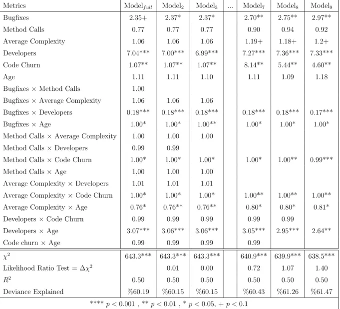
In our work, the selection of confounders is based on earlier findings and the results of the pairwise correlation to eliminate high collinear confounders. We add the interaction of the confounders in the model. Multicollinearity diagnosis test is used to test the initial model which contained confounders and interactions. Then, the final model is achieved based on a backward fashion, starting with the highest order term (interaction). A goodness of fit model was applied to confirm that the elimination of each interaction does not affect the reduced model. Another goodness of fit test was also applied to the final model, which was not done in other previous related works. The motivation and the methodology of this work are covered in details in Chapter 3.
2.2
Explanatory Work on Software Development
Ef-forts
Earlier research on prediction of software development efforts was based on three ap-proaches. The first approach was based on expert judgment in estimation [64, 65, 66, 67]. The purposes of that research was to build accurate models based on expert judgment and compare them with mathematical and machine learning models. The second approach was to use a mathematical model to estimate the effort [68, 69, 70, 71, 72]. The most common mathematical model is the COCOMO model [72], which uses the size of a project (measured in thousands of coded lines) as the main parameter to estimate effort. The third approach
was based on modeling techniques and used either analogy-based models (e.g., [73, 74, 75]) or machine-learning models (e.g., [76, 77, 78, 79]). Most of the research used the third ap-proach because of its simplicity and low cost [80], specifically when applying several machine learning methods to improve estimation.
Because our work falls into the third category, we focus on the related studies that applied predictions to obtain an accurate estimation. Further, because we included interactions of metrics in our model, we highlight some related studies that involved interactions for prediction.
Angelis et al. [81] applied OLS on numerical and categorical data using ISBSG metrics. Missing values were treated by elimination the complete row (i.e., list-wise deletion). They used three numerical metrics: function points (Size), efforts, and max team size. The study transformed data to a logarithmic format to obtain normal distribution and implement OLS regression. The study used development-type and language-type metrics in a categorical format. The study applied a correlation test using χ2 values, and highly correlated metrics were eliminated. Briand et al [82] used OLS, ANOVA, CART, and analogy-based approaches as well as a combination of methods (CART with OLS and CART with analogy). They used the Laturi data set, which consists of 206 projects collected from companies from Finland. They found that size, organization type, and target platform are the top prediction metrics, and that the CART model performed better than other approaches for local or cross-company projects. A replicated assessment work [83] used the same approaches that were used in [82] with a multi organization software project data set. Size and maximum team size were the two major overriding variables in all models. The results of the replicated work showed that CART performed relatively poorly and the OSL model was sufficient to predict the effort. OLS was also used in several other studies [84, 85, 64, 86].
Several other studies applied machine learning algorithms to predict efforts [87, 78, 88, 89, 76, 90, 91, 92, 77, 93]. Some studies proposed or applied single method of prediction, and other applied several methods, ensemble methods, or methods applied on fuzzy decision tree.
Srinivasan and Fisher [87] applied regression tree and neural networks on COCOMO and Kemerer’s data sets and compared their accuracy with different arithmetical models such as COCOMO and Software Lifecycle Management SLIM. Kocaguneli et al. [75] proposed an analogy-based method that outperformed linear regression and neural network estimators. They applied the same method for the transfer learning methodology to estimate efforts. Kumari and Pushkar [91] proposed cuckoo Search algorithm and hybridizes it with neu-ral networks to improve the prediction of effort estimation. An estimation method based on fuzzy logic was proposed in [94], and it shewed a significant improvement in prediction compared to other studies. Sarro et al. [95] a genetic programming method on the Deshar-nais, Finnish, and Miyazaki data sets, and they measured their performances using MMRE, PRED(25), and MdMRE. The best results achieved for MMRE, MdMRE, and PRED(25) were 0.51 in Miyazaki, 0.43 in Desharnais, and 0.32 in Miyazaki and Desharnais. A causal discovery algorithm using a PC search algorithm was proposed in [79] to predict direct, in-direct, and bi-directed edges between software efforts metrics. Sigweni et al. [96] applied leave-one out cross validation method based on chronological orders of software projects (i.e., grow one at a time technique) and not based on random selection of projects for Desharnais and Finnish data set. The study found that the proposed technique is more realistic than the traditional method.
Baskeles et al. [89] applied neural networks, regression trees, and support vector regres-sion for the NASA and Turkish industry data sets. Li et al. [90] used Neural networks and regression trees on Desharnais and Maxwell data sets. Radinski and Hoffmann [76] applied twenty-three machine learning methods (e.g., Bayes, lazy, rules, and trees) on four datasets (i.e., COCOMO, Desharnais, Maxwell, and QQDefects) to predict software development effort. Andreou and Papatheocharous [78] used fuzzy decision trees to predict cost on the ISBSG data set. Huang et al. [88] proposed a model based on fuzzy decision trees for software cost prediction for the COCOMO dataset. Kocaguneli et al. [97] applied ensemble methods combining multiple learners with multiple preprocessing method and found that CART re-gression ranked at the top. Elish [93] applied ensemble learning method using five classifiers on five data sets. The result of the ensemble method outperformed the performance of indi-vidual classifiers. Another ensemble method was developed by [98] and the study found that
applying principle component analysis with the CART regression was ranked at the top of all other methods. Several machine learning methods (i.e., k-NN, support vector regression, multilayer perceptron, and decision trees) were applied in [92]. Nassif et al. [77] applied four types of neural networks (i.e., multilayer perceptron, general regression neural network, radial basis function neural network, and cascade correlation neural network) on ISBSG data set. Jodpimai et al. [99] applied five data preprocessing techniques with five learning techniques (i.e., regression analysis, support vector regression, classification and regression tree, k-NN, and radial basis function). The study did not find a dominant learning that outperformed all other algorithms.
In the area of software effort estimation, ordinal regression has been used once by [100]. In this study, the models were built for prediction and used on three data sets: Maxwell, CO-COMO81, and ISBSG. The study used both categorical and numerical independent metrics. The authors log transformed the size and duration metrics to gain normality in the distri-bution. The response confounder, effort, was discretized to four levels in all data sets using the equal frequency method. The learning model was developed using forty-two projects to test ten projects. The authors evaluated the model using MMRE, PRED(25), hit rate, and correct classification.
Some studies have considered the effect of metrics when they interact with each other. Interactions were considered with a goal to improve the prediction. Three studies have used interactions in prediction models [101, 102, 103].
Gray et al. [103] used logistic regression for three response metrics related to the over-estimation, underover-estimation, and error estimation. For every model, the study developed all possible scenarios including interactions of metrics. The goal of adding interaction was to get the best fit model according to the Akaike information criterion (AIC). For all the scenarios involving the three models, interactions did not improve the fit. Tsunoda et al. [101] aimed to determine whether interactions can change accuracy by comparing them to models without interactions. The study emphasized the necessity of using interactions to improve prediction. However, not enough evidence was shown to prove the case. A slight
improvement in performance occurred with NASA data set when the model used interac-tions. Tsunoda et al. [102] investigated the role of moving windows in estimating efforts. This involved interactions between size and timing (the age of the project). The results of the interaction showed a slight improvement in the evaluation criteria for some cases.
Missing values are very common in software development estimation. Next, we highlight the major treatments applied by studies in this field and their main findings. Strike et al. [85] evaluated the use of several techniques: listwise deletion, mean imputation, and eight different types of hot-deck imputation. The study found that hot-deck imputation perform consistently with the highest precision and least bias compared to other techniques. k-NN achieved better performance than toleration and mean imputation techniques in [104]. Another study [105] suggested the use of multinomial logistic regression over listwise deletion, mean imputation, regression imputation, and expectation maximization for missing data treatment with ISBSG projects. Song et al. [106] found k-NN to improve prediction models built using the C4.5 algorithm. The study also found that the percentage of the missing data should not exceed 40%. Idri et al. [107] studied three techniques of missing data treatment (i.e., toleration, deletion, and k-NN) using two types of analogy models. The study found that using k-NN can improve the performance of the models more than using toleration and deletion.
Our proposed approach (in Chapter 5) shares a similar goal, which explains how specific metrics and interactions contribute to the software effort. The involvement of the interactions should add more explanations from the model unlike related works. In addition, we use a holistic approach that includes a test for correlation, discretization of numerical data, handling of missing values, multicollinearity, elimination of insignificant interactions and metrics, and goodness of fit. The methodology and implementation of the three case studies of different datasets are explained in details in Chapter 5.
2.3
Related Works on Causality
Structural equation modeling (SEM) has not been used in the field of software engineer-ing or in any closely related areas. However, this method has been used in many other areas such as psychology (e.g., [11, 108, 109]), education (e.g., [110]), biology (e.g., [111]), neuroscience (e.g., [112]), ecologic studies (e.g., [113]), accounting (e.g., [114]), marketing (e.g., [115, 116]), hospitality management (e.g., [117]), operations management (e.g., [118]), management information systems (e.g., [119]), and strategic management (e.g., [120]).
In [11], the SEM methodology was described as a guide for researches in psychology. Martens [108] reviewed 99 papers published in the Journal of Counseling Psychology be-tween 1987 and 2003. The study analyzed how researchers handled issues such as normality and goodness of fit. For example, in nineteen percent of studies the authors discussed the normality of their data. The goodness of fit test using χ2 was the most common approach, reported by ninety percent of the studies. A comparative fit index (CFI) was used by sixty percent of the studies, the Tucker-Lewis index (TLI) was used by forty-three percent of the studies, and the root mean square error of approximation (RMSEA) was used by thirty-eight percent of the studies. In the same domain, an earlier study [109] reviewed seventy-two papers between 1977 and 1987.
Hair et al. [120] analyzed more than a hundred papers published in top-ranked journals between 2000 to 2011 in the field of strategic management. The range of the number in-dependent variables used in the surveyed papers was from seven to 114. The range of the number of latent variables used in these papers was from two to thirty-one. The number of variables per latent variable ranged from one to ten, with a median equal to three variables. This indicates that more than fifty percent of the studies used no fewer than three variables per latent variable, which is the recommended number.
Hair et al. [116] analyzed 204 studies published in the last thirty years in top-ranked journals in the marketing field. The range of the number of latent variables was from two to twenty-nine, with a median of seven. The number of variables per latent variable ranged from one to twenty-seven, with a median of four. The total number of variables used in the sample of papers ranged from four to 131, with a median of twenty-four. Henseler et
al. [115] addressed the specific requirements and typical research problems of international marketing using path modeling techniques. In the business intelligence field, Jakli et al. [121] used partial least squares (PLS) in an SEM model to analyze the interrelated role of compatibility in predicting business intelligence and analytics, finding that compatibility perceptions have a direct positive impact on use intention.
Kaufmann and Gaeckler [122] analyzed seventy-five papers published in top-ranked jour-nals between 2002 and 2013 in the field of supply chain management. The number of latent variables in analyzed studies ranged from three to twenty-one, with a median of six. The number of structural model relations (i.e., relations between latent variables) ranged from three to twenty-five with a median of eight.
Ringle et al. [119] surveyed 109 papers from journals on information technology and management information system. The number of latent variables used in these studies went from three to thirty-six, with a median of seven. The number of structural models relations ranged from two and sixty-four, with a median of eight. The median number of variables used with every latent variable was three. The total number of independent variables ranged from five to 1,064, with a median of twenty-six independent variables.
Ali et al. [117] reviewed hospitality management journals published from 2001 to 2015. A total of twenty-nine papers were reviewed in this study. The sample sizes used in reviewed studies ranged from 106 to 1,500 observations. The number of latent variables ranged from three to twenty, with a median of seven. The number of structural paths ranged from three to twenty-four, with a median of six. The total number of independent variables ranged from twelve to seventy-eight, with a median of twenty-two.
Peng and Lai [118] reviewed forty-two papers from the top eight journals in operations management field. The sample size for all papers ranged from thirty-five to 3,926 obser-vations. In the management field, Kulikowski [123] applied SEM and found a direct rela-tionship between pay for individual performance and work engagement. Additionally, the authors found an indirect relationship between the two factors through pay satisfaction.
Causal modeling using SEM has not been used in the software engineering field. However, some related works used BN for prediction, network structure, and decision-making [124, 125, 126, 127, 43, 128, 129]. BN are famous of their ability to predict causal relationships for continuous and discrete variables. Here, we discuss the studies in the field of software fault proneness prediction, which was also discussed earlier.
Fenton et al. [124] reviewed methods used for software fault proneness prediction and suggested using the BN method. The authors claimed that software faults are influenced by other factors that are not related to code complexity, such as the difficulty of the problem and analyst skill. In addition, using causal models could help understanding software faults at every stage of the software development because the cost of defects differ at every stage. The researchers also introduced a prototype model to explain how BN prediction can be implemented. The study built a model with two stages of software development: the first stage covers specification, design, and coding, and second stage covers the testing phase. Another work by Fenton et al. [125] encouraged the use of BN to predict models to support effective risk management and decisions. The researchers claimed that reliance on regression model is not enough to explore all causal effects on software quality. In a follow up work, Fenton et al. [126] used BN as a general approach that can be applied to any lifecycle, which helped for decision-making purposes. The method was built to overcome the limitation of earlier work [124, 125] by avoiding a separate model for each development lifecycle. The general model can detect specification, development defects, and testing defects. Fenton et al. [128] used BN to predict software defects and software reliability. The study emphasized that any model using defects in one phase to predict defect at subsequent phase should incorporate causal factors such as testing and quality levels. Therefore, the study applied BN to predict post-release defects and reliability, taking into account the design process quality and testing quality levels. The study [128] also used dynamic discretization approach to improve the accuracy of software defect prediction.
Wagner [130] transferred the activity based quality models (ABQM) [131] to a BN model. The main aim of the model was to provide quality managers with a systematic method to conduct assessment and prediction. The study proposed a four-step approach for transferring activity-based quality models to BN network. The four steps can be summarized as follows:
(1) define the activity that was intended to be measured (e.g., maintenance), (2) define facts and activities that are related, (3) add additional variables related to facts and activities, (4) apply BN to predict the outcome of the model. The study pointed out that it is necessary to answer questions like what variable is more important than others, which we trying to address in this work and from our previous attempts of the explanatory work.
Other studies used BN for software fault proneness and reliability prediction [127, 43, 128, 129]. Van Koten and Gary [129] constructed a BN model using object-oriented metrics for software maintainability prediction. The model was compared with other regression tree and multiple regression models, and used absolute residual, magnitude of relative error MRE, and pred measures to compare performance of all models. The study found BN model outperformed the regression tree and multiple regression models. Pai et al. [127] realized the importance of validating relationship of performance measures with external quality metrics. The study built a model using two response variables (i.e., fault proneness and fault content) and seven independent variables from the object-oriented static code metrics [127]. The study did not consider direct effect between independent variables and the response variables, and did not consider the indirect effect. Okutan and Olcay [43] used object-oriented metrics on Promise data repository to predict software fault proneness. The study built a causal model for every data set used based on score system of association between every pair of metrics. The study eliminated metric based on the score result, which suggested no association of the eliminated metrics with any other metric. The study showed some of the direct and indirect effects between some of the object-oriented metrics used. The study did not include change metrics which would increase more complexity to each model. The study also did not consider the high correlation and multicollinearity of the model.
A benchmark analysis study [40] was conducted using twenty-two classifiers on ten NASA MDP datasets. The performance of BN in the study was among that of the top six classifiers in terms of the area under the curve (AUC). BN followed random forest, neural networks MLP1 and MLP2, and support vector machines LS-SVM and L-SVM. The performance of BN had no statistically significant differences from those of higher-ranked classifiers. Another benchmark study [41], which focused only on BN classifiers, applied fifteen BN classifiers
to predict software fault proneness using eleven NASA MDP data sets [41]. The study compared the performance of all classifiers using the ROC curve and H-measure metrics. They found that augmented naive Bayes classifiers performed similarly or better than naive Bayes classifier.
Some studies have combined SEM with other approaches to replace the estimation from the traditional ML to BN or to take advantage of the prediction ability of BN algorithms (e.g., [132]). Further, some studies have applied neural network prediction on SEM networks. To use neural networks, the causal network should consist only of measured variables. In other words, latent variables are not allowed in neural networks. Therefore, the SEM should not contain any latent variable, to be applicable for neural network prediction.
SEM and the Gibbs sampling using the Markov chain Monte Carlo (MCMC) method was applied in [133]. The study estimated the parameters using the Gibbs sampling instead of the maximum likelihood ML, the estimation method that is normally used with SEM. The integration of SEM and BN appeared in [132]. The study proposed a causal model for management decision support that links SEM and BN, with a goal to examine the factors that cause customer retention. The prediction accuracy performance gained from the BN models varied from seventy-four to ninety-three percent. Another study [113] linked SEM and BN to explore the effects of environmental factors on freshwater macroinvertebrates. The causal network was built using the SEM concept, and BN was used for prediction and decision-making. Another attempt to combine SEM with prediction via neural networks was made in [134]. The SEM diagram of the model included only measured variables (i.e., no latent variables were included) and one response variable, which measured consumer intention to adopt mobile commerce. Therefore, using the same model for neural network algorithms was explored for prediction. A similar approach was employed by [135] to measure the adoption of inter-organizational systems. Another similar approach was implemented by [136] to measure the customer satisfaction and loyalty with respect to airline services.
In our study, we used software fault proneness case study, which had thirty variables from static code and change variables. Moreover, these variables were extracted at a single point of the development cycle. Therefore, building a network using BN methodology would result in a very complex model and very hard to explain. Our focus is to build an explanatory causal
model which can be fulfilled by using structural equation modeling. Thus, we used only the statistical methods and regression analysis associated with SEM methodology, data analysis, sampling, variable selection, latent variable creation, model specification, model estimation, and model validation. Latent variables gave us an advantage to simplify the model and reduce the number of paths that would result without using them. Also, we considered the high correlation of selected variables to ensure that under every model, no high correlation is detect between any pair of variables. Further, we analyzed the multicollinearity of the linear model using all variables. The detailed methodology, and the case study are explained in Sections 6.2 and 6.3, respectively.
Chapter 3
Using a Case-control Study to
Explain Software Fault Proneness
This chapter implements an explanatory work to explain software fault proneness. For that, several steps are established to build a model that fit the data and to explain con-founders that contribute to the software faults. In this chapter, a matched study using case-control methodology is suggested to build the explanatory model. Further, the mod-els include interactions between confounders to assess how they add to the model with the main confounders. The main motivation for this work is that there is a need to use a proper method to measure the effect of the main confounders and their interactions, consider the stratification in the analysis, consider the multicollinearity of the model, and eliminate the interactions and confounders that do not statistically harm the model. The proposed methodology is explained in details in Section 3.2, after highlighting on the contribution of this work in Sections 3.1. First, we used Eclipse’s Europa as a case study, and then the work was replicated using Ganymede in Section 3.3. The work was also replicated on projects from the Apache software foundation (i.e., Derby, Ant, and Xalan), which is presented in Section 3.4. We provided explanation of the results of all projects in Section 3.5. At the end, the threats of validity of this work are discussed in Section 3.6, and the chapter is concluded in Section 3.7.