A New Deep Generative Network for
Unsupervised Remote Sensing Single-Image
Super-Resolution
Juan M. Haut,
Student Member, IEEE,
Ruben Fernandez-Beltran, Mercedes E. Paoletti,
Student
Member, IEEE,
Javier Plaza,
Senior Member, IEEE,
Antonio Plaza,
Fellow, IEEE,
and Filiberto Pla
Abstract—Super-resolution (SR) brings an excellent op-portunity to improve a wide range of different remote sensing applications. SR techniques are concerned about increasing the image resolution while providing finer spatial details than those captured by the original acquisition
This paper has been supported by Ministerio de Educaci´on (Res-oluci´on de 26 de diciembre de 2014 y de 19 de noviembre de 2015, de la Secretar´ıa de Estado de Educaci´on, Formaci´on Profesional y Universidades, por la que se convocan ayudas para la formaci´on de profesorado universitario, de los subprogramas de Formaci´on y de Movilidad incluidos en el Programa Estatal de Promoci´on del Talento y su Empleabilidad, en el marco del Plan Estatal de Investigaci´on Cient´ıfica y T´ecnica y de Innovaci´on 2013-2016. This work has also been supported by Junta de Extremadura (decreto 297/2014, ayudas para la realizaci´on de actividades de investigaci´on y desarrollo tecnol´ogico, de divulgaci´on y de transferencia de conocimiento por los Grupos de Investigaci´on de Extremadura, Ref. GR15005). This work has been additionally supported by the Generalitat Valenciana through the contract APOSTD/2017/007 and by the Spanish Ministry of Economy under the project ESP2016-79503-C2-2-P. ( Corresponding author: J.M. Haut.)
J. M. Haut, M. E. Paoletti, J. Plaza and A. Plaza are with the Hyper-spectral Computing Laboratory, Department of Technology of Com-puters and Communications, Escuela Polit´ecnica, University of Ex-tremadura, PC-10003 C´aceres, Spain.(e-mail: [email protected]; [email protected]; [email protected]; [email protected]).
R. Fernandez-Beltran and F.Pla are with the Institute of New Imaging Technologies, University Jaume I, 12071 Castell´on, Spain. (e-mail: [email protected]; [email protected]).
instrument. Therefore SR techniques are particularly use-ful to cope with the increasing demand remote sensing imaging applications requiring fine spatial resolution. Even though different machine learning paradigms have been successfully applied in SR, more research is required to improve the SR process without the need of external High-Resolution (HR) training examples. This work proposes a new convolutional generator model to super-resolve low-resolution (LR) remote sensing data from an unsupervised perspective. That is, the proposed generative network is able to initially learn relationships between the LR and HR domains throughout several convolutional, down-sampling, batch normalization and activation layers. Then, the data are symmetrically projected to the target resolution while guaranteeing a reconstruction constraint over the LR input image. An experimental comparison is conducted using twelve different unsupervised SR methods over different test images. Our experiments reveal the potential of the proposed approach to improve the resolution of remote sensing imagery.
Index Terms—Remote sensing, super-resolution, convo-lutional neural networks.
I. INTRODUCTION
Remote sensing image acquisition technology is un-der constant development and now provides improved
imagery that are useful to tackle new challenges and needs [1]. Nonetheless, the increasing demand of highly accurate remote sensing imaging applications, such as fine-grained classification [2], [3], target recognition [4], [5], object tracking [6], [7] or detailed land monitoring [8], still makes the spatial resolution of optical sensors one of the most important limitations affecting remotely sensed imagery. In general, the spatial resolution of an instrument defines the pixel size covering the Earth surface and, therefore, it describes the ability of the sensor to capture small image details. Even though the most technologically advanced satellites are able to discern spatial information within a squared meter on the Earth surface [9], the high cost of this acquisition technology, together with the light physical limitations when substantially decreasing the sensor pixel size, are usually important constraints that make algorithmic-based resolution enhancement techniques an excellent tool for remote sensing imaging applications [10].
The general objective in super-resolution (SR) [11]– [14] is to improve the image resolution beyond the sensor limits. That is, increasing the number of image pixels while providing finer spatial details than those captured by the original acquisition instrument. Depending on the number of input images, it is possible to distinguish between two kinds of SR methods, single-image [15] and multi-image [16]. Whereas single-image SR techniques use a single image of the target scene to obtain the super-resolved output, multi-image SR methods require several scene shots simultaneously acquired at different positions. In remote sensing, the single-image approach is usually adopted because it provides a more general scheme to super-resolve any kind of imaging sensor without the need for a satellite constellation [17], [18].
The single-image SR approach can be considered as an ill-posed problem since there is not a single solution for any given low-resolution pixel, i.e. the solution is
not unique. This fact has been traditionally mitigated by constraining the space of possible solutions using a strong prior information extracted from a specific set of images. In this sense, artificial neural networks (ANNs) have become a powerful tool due to their ability to learn image priors from any given dataset. Traditionally used in the pattern recognition fied [19], ANNs have been also intensively used for the analysis of remotely sensed imagery [20]–[22], reaching a good performance without prior knowledge on the input data distribution and offering multiple training techniques.
With the great evolution of deep learning [23], [24] (DL) techniques, the ANN architecture has evolved from the simple linear perceptron classifier to deeper architectures (multilayer stack of simple modules) called deep neural networks (DNNs), allowing to create more complex models which can extract more abstract infor-mation (features) from the data than shallow ones [25]. DNNs are currently able to perform SR in a successfully way [26]. In particular, convolutional neural networks (CNNs) [23] stand out as a powerful image processing tool due their effectiveness, especially for the analysis of large sets of two-dimensional images. CNNs have proven to produce high performance in a great variety of tasks, such as image analysis and target detection [27]– [30], pan-sharpening [31], [32], reconstruction of remote sensing imagery [33] and also image SR [34]–[38]. How-ever, these supervised techniques require sufficient high-resolution (HR) training examples in order to perform properly and generalize well. In addition, they usually tend to over-fit quickly due to the models’ complexity and the lack of training data. Note that obtaining rele-vant remote sensing training data is expensive and time consuming. Besides, the amount of available training remote sensing datasets is rather limited, and normally they suffer from a lack of image variations and diversity. For these reasons, supervised learning is difficult to carry
out, while unsupervised learning methods do not need any external data to train. On the other hand, the CNN is a very flexible model that can be adapted to different learning models, such as convolutional autoencoders (AEs) [39], [40], convolutional deep belief networks (DBNs) [41], convolutional generative adversarial neural networks (GANs) [42], convolutional recurrent neural networks (CRNN) [43] or fully convolutional networks (FCN) [44], among others. In particular, we highlight the hourglass network [45], [46], whose topology is symmetric, related to the convolution-deconvolution ar-chitecture, and also to the encoder-decoder, characterized by a first step of pooling down to a low resolution (composed by convolutional and max pooling layers) and a second step of upsampling to a higher resolution and combining features across multiple resolutions.
Following thehourglassapproach, a new unsupervised neural network model is proposed in this work in order to super-resolve remote sensing images. The novelty of the proposed approach lies on using a generative random noise to introduce a higher variety of spatial patterns which can be promoted to a higher scale throughout the network according to a global reconstruction constraint. Even though the relevance of generating new spatial variations when super-resolving remotely sensed data in a unsupervised manner, this is, to the best of our knowl-edge, the first time an unsupervised generative network model has been successfully formulated to super-resolve remote sensing imagery. Specifically, a convolutional generator network has been adopted, where from a given image XLR ∈ RC×W×H, a higher resolution version XHR ∈ RC×t·W×t·H is generated (being W < t·W
andH < t·H, witht being a factor of resolution).
In addition, the algorithm has been adapted to be effi-ciently executed in parallel on graphics processing units
(GPUs)1 and presents some methodological
improve-ments to make the model more efficient and effective. To summarize, the main contributions of this work can be highlighted as follows:
• An hourglass convolutional neural network model is developed to perform unsupervised super-resolution.
• In particular, a convolutional generator model has
been implemented to super-resolve low-resolution remote sensing images.
• Starting from generative random noise, the model is able to reconstruct the image, promoting it to a higher scale according to a global reconstruction constraint.
• Experiments over three datasets, with 2 scaling factors and 12 different SR methods, reveal the competitive performance of the proposed model when super-resolving remotely sensed images. The remainder of the paper is organized as follows. Section II presents an overview of single-image SR methods and their limitations. Section III describes the methodology employed by the proposed convolutional generator model. Section IV validates the proposed ap-proach by performing comparisons with different single-image SR methods. Finally, Section V concludes the paper with some remarks and hints at plausible future research lines.
II. BACKGROUND
A. Brief single-image SR overview
Broadly speaking, single-image SR algorithms can be categorized into three different groups [53], [54]: image
1The use of high performance computing methods (HPC), including parallelization with accelerators such as field programmable gate arrays (FPGAs) and GPUs [47]–[49], or the distribution with clusters and clouds [50], [51], have demonstrated great utility for the classification of remote images [52].
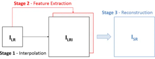
Fig. 1. Super-resolution based on image reconstruction (RE).
reconstruction (RE), image learning (LE) and hybrid (HY) methods. RE methods aim at reconstructing HR details in the super-resolved output assuming a specific degradation model along the image acquisition process, which is typically defined by the concatenation of three operators: blurring, decimation and noise. Therefore, RE methods can be usually defined in terms of the three following stages (Fig. 1): Stage 1, where the LR input image (ILR) is upscaled to the target resolution (ILRI) using a regular interpolation kernel function. In Stage 2, some physical features are extracted fromILRto estimate
the singularities of the spatial details. Finally, Stage 3 aggregates both the interpolated image (ILRI) and the
extracted LR features to obtain the final reconstructed resultISR.
Each particular RE method makes its own assumptions about the imaging model and the reconstruction process to relieve the ill-posed nature of the SR problem. Some of the most popular RE approaches are iterative back projection (IBP) [55], gradient profile prior (GPP) [56], and point spread function (PSF) deconvolution [57]– [59]. The rationale behind IBP is based on iteratively refining an initial interpolation result by means of min-imizing the reconstruction error between the LR input image and a simulated low-resolution version of the super-resolved result. GP takes advantage of the fact that the shape of the gradient profiles tends to remain invariant across scales, therefore LR gradient can be used to reconstruct the output image sharpness. PSF
deconvolution methods tackle the upscaling problem from a deblurring point of view, that is, they initially estimate the imaging model PSF and then they try to remove the interpolated image blur.
Regarding LE methods, this type of techniques are able to provide a more powerful SR scheme because they learn the relationships between LR and HR domains from an external training set containing ground-truth HR images. As Fig. 2 shows, RE methods can be divided into three stages: In Stage 1, the relations between LR and HR components are learned from a specific training set. Stage 2 aims at estimating the HR components that are related to the LR input image structures. Finally, Stage 3 combines the estimated HR components to generate the final super-resolved result. Over the past years, different machine learning paradigms have been successfully applied in LE-based SR. Sparse coding [60], neighborhood embedding [61] and mapping functions [62], [63] are among the most popular methods. In a nutshell, sparse coding-based techniques take advan-tage of the fact that natural images tend to be sparse when they are characterized as a linear combination of small patches. The neighborhood embedding approach assumes that small image patches of LR images describe a low-dimensional non-linear manifold with a similar local geometry to their HR counterparts. Mapping-based techniques cope with the SR task as a regression problem between the HR and LR domains.
Lastly, HY techniques work towards reaching an agreement between RE and LE approaches. In particular, they perform a training process but only using the LR input image. The rationale behind HY methods is based on the patch redundancy property pervading natural images, which assumes that natural images tend to contain repetitive structures within the same scale and over scales as well. Taking this principle into account, it is possible to find patches which appear in a lower scale,
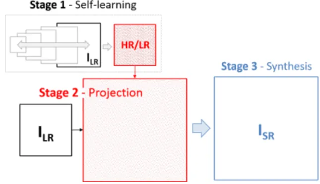
Fig. 2. Super-resolution based on image learning (LE).
without any blurring or decimation, and then extracting their corresponding HR counterparts from the higher scale image. Eventually, the super-resolved image can be generated using the LR/HR relationships learned across scales. In particular, HY methods generally follow the scheme shown in Fig. 3: In Stage 1, the self-learning process is conducted, that is, several lower scale images are initially generated from ILR and then those patches which tend to appear across scales are extracted. Stage 2 projects the input LR image to the target resolution using the relations previously learned. Finally, the final super-resolved result is generated in Stage 3 considering some sort of reconstruction constraint.
Logically, each specific HY approach defines its own assumptions about the imaging model and the patch searching criteria. For example, the work presented in [64] approximates the blur operator by a Gaussian kernel and the patch redundancy process is conducted by an approximation of the nearest neighbor search. Other works propose different kinds of modifications over this scheme. It is the case of [65] which introduces a model extension to enable patch geometric transformations across scales. Therefore, the number of patch matches can be increased and consequently the amount of learned LR/HR relationships. In other works, such as in [66], the blur operator is estimated at the same time as the SR
output is generated through an optimization process.
B. SR limitations in remote sensing
Each single-image SR methodology has shown to be particularly effective under specific conditions [15], [54]. RE methods are able to reduce the noise as well as the blur and aliasing inherent to interpolation kernel functions. However, the lack of relevant high-frequency information in the LR input image limits their effectiveness to small magnification factors, which can be an important limitation for many of the currently operational (moderate) resolution satellites [67].
LE-based techniques potentially overcome these draw-backs by learning the relationships between LR and HR domains from an external training set. Nonetheless, the availability of suitable HR training examples can also be a serious constraint for many satellites. Note that ground-truth HR images are usually not available in real sce-narios, and this may lead to an unrepresentative training phase with a biased super-resolved result. Eventually, the application of LE-based SR methods in actual ground segment production environments is rather limited [68]. HY methods offer the advantage of not requiring any external training set to learn the LR/HR relationships by taking advantage of the patch redundancy property over scales. However, the probability of finding patches
isfying this property decreases with the input resolution, and therefore the amount of useful LR/HR connections over scales highly depends on the input image.
With all these considerations in mind, unsupervised RE and HY methods are especially attractive to remote sensing. While supervised approaches use a training set of HR images to learn the relationships between the LR and HR domains [69]–[71], unsupervised approaches only make use of the target LR image to generate the corresponding super-resolved output result. Moreover, supervised network architectures implement a regressor function to project general LR image patches onto the HR domain. However, in a real-life remotely sensed data production environment there is not actual HR captured by the sensor. In this sense, unsupervised methods do not require the availability of HR images to train a general SR model, super-resolving each specific LR input image without using any other external data and providing the opportunity to offer new super-resolved data products in satellite and airborne missions that use relatively inexpensive sensors without the need of using any external HR training set. Nevertheless, the number of works in the remote sensing literature dealing with the unsupervised SR problem is rather constrained, and this is precisely the gap that motivates this work.
In [72], authors propose a SR approach using a back-propagation neural network as a regression function, and basing on (i) spectral unmixing, (ii) super-resolution mapping and (iii) self-training, which is exploited taking advantage of the embedding provided by the spectral unmixing process itself. However, this approach could be highly affected by the spectral simplex geometry of the input image [73]. In contrast, a hybrid (also called self-learning) SR scheme has been proposed in this work to super-resolve remote sensing data from an unsupervised perspective, basing on a new end-to-end convolutional generator model. The rationale behind the
proposed approach is based on learning the relationships between the LR and HR domains by down-sampling the original input image to a lower scale and then using the learned relations at a lower scale to project the LR input image to the target resolution. However, the amount of spatial information that it is possible to retrieve from a down-sampled LR image may be limited, so a random generative noise has been additionally introduce together with a global reconstruction constraint to activate a higher amount of consistent spatial variations along the SR process. That means, random spatial variations are initially generated to be introduced in the self-learning process in order to mitigate the ill-posed nature of the SR problem. Regarding the proposed network global scheme, it provides a similar end-to-end framework to other deep learning-based approaches, e.g. [69]–[71], where the original LR image is used to learn the down-sampling filters at the same time that they are also used to generate the super-resolved output.
III. METHODOLOGY
Traditionally, a generator network is an algorithm for image generation, where given a random variablez, the model is able to learn internal relationships (represented by the model parameters θ) to generate an image X = fθ(z), i.e. a regression problem. This allows us to learn the distribution of the data and the correlations betweenz
andX. We can follow this approach in order to perform SR over remote sensing images, wherez∈RC×W×H is
random noise and X ∈R3×W
0×H0
is the desired RGB high resolution image.
Given a LR imageXLR∈R3×W×H the SR’s goal is
to improve the image resolution beyond the sensor limits obtaining a HR versionXHR∈
R3×t·W×t·HfromXLR,
wheretis the resolution factor andW < t·W,H < t·H. In order to do this, a deep model based on CNNs has been implemented. This kind of networks are composed
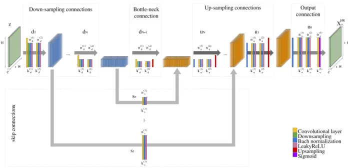
Fig. 4. The proposed 2D-CNN architecture model follows a symmetric topology. The input imagezgoes through a first step of down-sampling composed by blocks (d(1), d(2), ..., d(N)) of several CONV, down-sampling, BATCH-NORM and activation layers, where eachn(j)
d andk
(j)
d (withj= 1,2) are the number of filters and kernel sizes of each down-sampling connectiond(i). Then, symmetrically, data goes through the
up-sampling step, where the output of each blocku(i)(with number of filtersn(j)
u and kernel sizek(uj),j= 1,2and composed by CONV, BATCH-NROM, up-sampling and activation layers) is combined with the features of the correspondingdithrough a skip connectionsi, which also has a number of filtersn(1)s and a kernel sizeks(1)and is composed by a CONV, a BATCH-NORM and an activation layers.
by layers that are applied over defined regions of the input data, i.e. they are local-connected to the input, transforming the input volume to an output volume of neuron activations which will serve as input to the next layer. The fact that each layer is not completely con-nected to the previous layer (only with a patch/window defined as the receptive field) is a great advantage for data analysis, reducing the number of connections in the network, where each layer composes feature extraction stages working as a filter or kernel over patches of the input volume.
Depending on the treatment of the data, CNNs can be classified into three categories. Supposing thatx(i)∈
RC= [x(1i), x (i) 2 , ..., x
(i)
C]is a pixel withCspectral bands of imageX∈RC×W×H, withi= 1,2, ..., W·H, while P(j) ∈
Rb×p×p is a patch of X, where p is the width
and height (withp≤W andp≤H) andb the number
of spectral bands of the patch (with b ≤ C). 1D-CNN models take separately as input data each pixels vector
x(i), extracting only spectral information [74]. On the
other hand, 2D-CNNs extract spatial information, taking as input data the entire image X [75] or image patches
P(j)[76], whereCandbare set to small values, i.e. the
spectral information is not very relevant compared to the spatial information. Finally, 3D-CNNs extract spectral-spatial information, taking normally as input data patches
P(j) of the original image X [29], [30], where C and
b are set to large values, i.e. the spectral information is very relevant and it is combined with spatial information. Usually, for panchromatic and RGB remote sensing images, a 2D-CNN approach is taken while 1D- and 3D-CNNs are usually for multi- and hyperspectral images. This paper works with RGB remote sensing datasets, so a 2D-CNN architecture has been implemented to take
advantage of the spatial information contained in the images. It is composed by five different kinds of layers, described below:
• Convolution layer (CONV): this kind of layer is composed by a block of neurons where each slice (also called filter or kernel) shares its weights and biases between all the neurons that compose it. Given a CONV layer C(i), its output volume O(i)
(also called feature maps) can be calculated follow-ing equation 1 as the dot product between the n(i)
slices’ weightsW(i)and biasesB(i)(beingn(i)the number of depth slices, also known as number of filters or kernels) and a small region of the input volume O(i−1), i.e. a rectangular section of the
previous layer C(i−1), defined by the kernel size k(i) of the current layerC(i):
O(i)= (O(i−1)·W(i))f,l+B(i)= k(i) X m=1 k(i) X n=1 o(fi−−m,l1)−n·wm,n(i) +B(i) (1)
being o(f,li−1) the feature (f, l) of the feature map
O(i−1) ∈ RW,H, with f = 1,2, ..., W and l = 1,2, ..., H, and w(m,ni) the weight(m, n)of weight matrixW(i)∈Rk (i),k(i) . As result, O(i) ∈ Rn (i),W0,H0
forms a data cube whose depth is defined by the number of kernels
n(i) (that indicates the number of output feature
maps) and its width and height are calculated as:
W0 =(W k+ 2P)
S + 1 andH
0 =(Hk+ 2P)
S + 1
respectively, whereP indicates the padding (zeros) added to the input data borders andS indicates the stride of the kernel over the data. W and H are respectively the width and height of the previous feature maps O(i−1)∈
Rn
(i−1),W,H
.
• Batch normalization layer (BATCH-NORM): nor-mally it is placed behind the convolution layer and
it applies the normalization defined by equation 2 over the batch data:
y= xp−mean[x]
Var[x] +·γ+β (2)
whereγandβare learnable parameter vectors, and
is a parameter for numerical stability.
• Activation layer: after CONV and BATCH-NORM layers, the activation layer or non-linearity layer embeds a non-linear function that is applied over the output of previous layer, as the rectified linear unit (ReLU) [77], [78]. In this case, the LeakyReLU function is implemented [79]: f(x) = x ifx >0 αx ifx≤0 (3)
where α is a small non-zero parameter, normally 0.001.
• Down-sampling/Up-sampling layer: the proposed model also implements down-sampling and up-sampling layers at certain locations of the archi-tecture. The first one reduces the spatial resolu-tion of the input volumes by reducing the width and height with a resolution factor t. A max pool function is generally implemented to perform the down-sampling, however the proposed model down-samples the input data setting the strides of certain CONV layers to S = 2. Additionally, the up-sampling layers try to reconstruct the data size using the bilinear function given a scaling factor. The proposed methodology provides a novel approach to effectively super-resolve remote sensing data from an unsupervised perspective. Specifically, our model receives the random noise-vectorz as input data, which is resized into a cube matrix RC×t·W×t·H in order
to feed the network, where W and H are the width and height of the original LR remote sensing image,
resolution factor. Following a fully-connectedhourglass
architecture [45], [80], z goes through two main steps composed by several blocks:
1) The down-sampling step is composed byN blocks of layers, called d(i) (i = 1,2, ...N), where the
input of each one is the feature maps of the previous one. Each d(i) is composed by an
ini-tial CONV layer Cd(1) that performs the down-sampling step by its stride S = 2, dividing the output volume size by two. This output volume feeds the BATCH-NORM layer and the non-linear LeakyReLU activation function. The output of the neuron activations feeds the second CONV layer
Cd(2) without down-sampling (i.e. S = 1) and also followed by a BATCH-NORM layer and the LeakyReLU activation function. Cd(1) and Cd(2)
have their own number of filters (n(1)d and n(2)d ) and their own kernel size (kd(1) andkd(2)). In fact, each block d(i) is reducing the space
information, i.e. generating a low spatial resolution data that will feed the second up-sampling step. 2) The up-sampling step is symmetric to
down-sampling one and it is also composed byN blocks of layers, calledu(i)(i=N, ...,2,1), where the
in-put of each one is the outin-put of the previous one. In this case, eachu(i)is composed by several stacked
layers. The first one is a BATCH-NORM layer, followed by the first CONV layer Cu(1) (which maintains the size of the data, i.e. S = 1) and its BATCH-NORM and LeakyReLU function. The output of the neuron activations feeds the second convolutional layerCu(2)(which also maintains the size of the data). After the BATCH-NORM and the activation function, the output will finally feed the bilinear up-sampling layer with factor equal to 2. Again, Cu(1) and Cu(2) have their own number of
filters (n(1)u and n
(2)
u ) and their own kernel size (ku(1) andk
(2)
u ).
Both steps, down-sampling and up-sampling, are sym-metrical and connected by skip connections, i.e. the input of each up-sampling block u(i) is combined with the
correspondingd(i)through the skip connections(i)(i= 1,2..., N) composed by a CONV layer Cs(1), with its number of filtersn(si)and its kernel sizek
(i)
s , a BATCH-NORM layer and the activation function, LeakyReLU. In fact, the output ofs(i)is concatenated to the input of
u(i). The chosen topology is depicted in Fig. 4. At the end of the topology, an output block is added, composed with a CONV layer and a sigmoid function at the end. As result, a HR imageXHR
o ∈R3×t·W×t·H is generated as output of the network.
In particular, the SR’s goal is to generate a HR image from a LR one, minimizing the following cost function:
minkφ(XHR)−XLRk2 (4)
In fact, our remote sensing datasets are composed by HR images. However, we cannot use them because they can-not be considered as ground-truth to perform SR. In or-der to solve this, a LR version is generated from each HR image by a down-samplerφ:R3×t·W×t·H →R3×W×H,
so XLR = φ(XHR). In our case the down-sampler φ has been implemented using Lanczos3 resampling [81], where pixels of the original imageXHRare passed into an algorithm that averages their color/alpha using sinc functions. With this LR version we can perform the SR task. However, the model is generating a HR image,
XHR
o . In order to solve this, the down-sampler function
φ is applied overXHR
o . At the end, equation 4 can be rewritten as:
minkφ(XHR)−φ(XoHR)k2→minkXLR−XoLRk2 (5) The cost function defined by equation 5 is optimized iteratively by the model via Adam optimizer [82]. The
proposed method is summarized in Algorithm 1. Also, in Fig. 8 we can observe the XoHR image generated by the model at each epoch.
Algorithm 1Unsupervised remote sensing single-image super-resolution algorithm
1: procedure SR MODEL(XLR,t) .
XLR ∈
RC×W×H original low resolution remote
sensing image, t resolution factor
2: z←Random noise with sizeC×t·W×t·H
3: repeat 4: XoHR←model net(z) 5: XoLR←φ XoHR . φis Lanczos3 6: loss=MSE(XLR, XLR o )
7: ADAM Optimizer(loss)
8: z←XoHR
9: untilReach maximum epoch
10: returnXHR o 11: end procedure
In order to test the proposed model, two networks have been implemented. The first one performs a 2x SR over a LR image XLR∈
R3×W×H, i.e. the resolution factor
is set to t = 2, obtaining a XHR ∈
R3×2·W×2·H HR
image, and the second one performs a 4x SR, i.e.t= 4
obtaining a XHR∈
R3×4·W×4·H HR image. Following
the scheme presented in Fig. 4, both models have been implemented with the topology described in Tables I and II.
A. Metrics
In order to compare the properties of the obtained
XoHRimage with regard to the original remote sensing imageXHR, several evaluation metrics have been used. For the sake of simplicity, we rename XHR
o =Xo and
XHR = X, being x(i)
o and x(i) the i-th pixels of Xo andX respectively.
TABLE I
NETWORK TOPOLOGY FOR2X SUPER-RESOLUTION. THE UP-SAMPLING PHASE HAS BEEN PERFORMED WITH A
SCALE-FACTOR SET TO2.
Block ID CONV ID Kernel size Number of kernels Stride
k(dj)/ku(j)/k(sj) n(dj)/n (j) u /n(sj) Down-sampling connections d(1) C (1) d 3×3 256 2 Cd(2) 3×3 256 1 d(2) C (1) d 3×3 256 2 Cd(2) 3×3 256 1 Bottle-neck connection d(3) C (1) d 3×3 256 2 Cd(2) 3×3 256 1 Up-sampling connections u(2) C (1) u 5×5 256 1 Cu(2) 1×1 256 1 u(1) C (1) u 5×5 256 1 Cu(2) 1×1 256 1 Output connections u(0) Cu(1) 5×5 256 1 Cu(2) 1×1 256 1 Cu(3) 1×1 3 1 Skip connections s(1) C(1) s 1×1 3 1 s(2) C(1) s 1×1 3 1
Following equation 6, wherensamples is the number of pixels of X andXmax andXmin are the maximum and minimum values of image X, respectively, the
normalized root mean square error(NRMSE) measures the distance between the data predicted by a model,Xo, and the original data observed from the environmentX
that we want to model.
NRMSE(X, Xo) = r 1 nsamples · Pnsamples i=0 x(i)−x(i) o 2 (Xmax−Xmin) (6)
Peak signal-to-noise ratio (PSNR) [83] represents a better image quality than NRMSE. This metric is defined as the standard index for SR, being MAXfthe maximum signal value that exists in the originalXimage. A higher PSNR value indicates that the reconstructed image Xo
TABLE II
NETWORK TOPOLOGY FOR4X SUPER-RESOLUTION. THE UP-SAMPLING PHASE HAS BEEN PERFORMED WITH A
SCALE-FACTOR SET TO2.
Block ID CONV ID Kernel size Number of kernels Stride
k(dj)/ku(j)/k(sj) n(dj)/n (j) u /n(sj) Down-sampling connections d(1) C (1) d 3×3 256 2 Cd(2) 3×3 256 1 d(2) C (1) d 3×3 256 2 Cd(2) 3×3 256 1 d(3) C (1) d 3×3 256 2 Cd(2) 3×3 256 1 d(4) C (1) d 3×3 256 2 Cd(2) 3×3 256 1 d(5) C (1) d 3×3 256 2 Cd(2) 3×3 256 1 Bottle-neck connection d(6) C (1) d 3×3 256 2 Cd(2) 3×3 256 1 Up-sampling connections u(5) C (1) u 3×3 256 1 Cu(2) 1×1 256 1 u(4) C (1) u 3×3 256 1 Cu(2) 1×1 256 1 u(3) C (1) u 3×3 256 1 Cu(2) 1×1 256 1 u(2) C (1) u 3×3 256 1 Cu(2) 1×1 256 1 u(1) C (1) u 3×3 256 1 Cu(2) 1×1 256 1 Output connections u(0) Cu(1) 3×3 256 1 Cu(2) 1×1 256 1 Cu(3) 1×1 3 1 Skip connections s(1) C(1) s 1×1 3 1 s(2) C(1) s 1×1 3 1 s(3) C(1) s 1×1 3 1 s(4) C(1) s 1×1 3 1 s(5) C(1) s 1×1 3 1 is of higher quality. PSNR(X, Xo) = 20·log10 MAXf RMSE(X, Xo) (7)
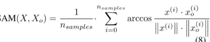
Spectral angle mapper (SAM) [84] calculates the angle between the corresponding pixels of the super-resolved imageXoand original imageX in the domain
[0, π]. SAM(X, Xo) = 1 nsamples · nsamples X i=0 arccos x (i)·x(i) o x(i) · x (i) o (8) The universal image quality index, also called Q-index, gathers three different properties in the image evaluation: (a) correlation, (b) luminance and (c) con-trast. Q(X, Xo) = nbands X j a z σ}| { IR σX σXo b z }| { 2X Xo (X)2 (X o)2 c z }| { 2 σX σXo (σX)2 (σXo) 2 j (9)
An extension of Q-index is the structural similar-ity (SSIM) [85], a well-known quality metric used to measure the similarity between two images. It is a combination of three factors (loss correlation, luminance distortion and contrast distortion).
SSIM(X, Xo) = (2µXµXo +c1)∗(2σXXo+c2) µ2 X+µ2Xo+c1 ∗ σ2 X+σX2o+c2 (10)
Erreur relative globale adimensionnelle de synthese
(ERGAS) [86] measures the quality of obtained Xo taking into account the scaling factor to evaluate the super-resolved image. ERGAS(X, Xo) = 100 nsamples v u u t 1 nbands nsamples X i=0 RMSE(x(i), x(i) o ) x(i) !2 (11) IV. EXPERIMENTS
A. Experimental Configuration and Datasets
In order to test the performance of the proposed model, several experiments have been conducted using two different hardware environments:
• A GPU environment composed by a 6th Genera-tion IntelR CoreTMi7-6700K processor with 8M of
Cache and up to 4.20GHz (4 cores/8 way multi-task processing), 40GB of DDR4 RAM with a serial speed of 2400MHz, a GPU NVIDIA GeForce GTX 1080 with 8GB GDDR5X of video memory and 10 Gbps of memory frequency, a Toshiba DT01ACA HDD with 7200RPM and 2TB of capacity, and an ASUS Z170 pro-gaming motherboard. The software environment is composed by Ubuntu 16.04.4 x64 as operating system, Pytorch [87] 0.3.0 and compute device unified architecture (CUDA) 8 for GPU functionality.
• A CPU enviroment composed by Intel Core i7-4790 @ 3.60GHz, 16GB of DDR3 RAM with a serial speed of 800MHz, a Western Digital HDD with 7200RPM and 1TB of capacity. The software en-vironment is composed by Windows 7 as operating system and Matlab R2013a.
It should be noted that our proposed method has been executed on the GPU environment, while the other methods have been executed in the CPU environment. Although our method uses Pytorch and CUDA, its par-allelization can still be further optimized and, therefore, the difference in computation times with regard to the other methods was not very significant.
Additionally, the employed database is composed by multiple RGB images from three different remote sens-ing repositories with the aim of testsens-ing the SR approach process under different sensor’s acquisition conditions and including different kinds of small perturbations. No additional levels of noise have been considered due to the design of the proposed SR approach, given by the noise-free scheme of Eq. 4, presented in other approaches such as [69]–[71], [88]. The employed repositories are described below, and are publicly available on this repos-itory2.
2https://github.com/mhaut/images-superresolution
1) UCMERCED [89]: It is composed by 21 land use classes, including agricultural, airplane, baseball diamond, beach, buildings, chaparral, dense resi-dential, forest, freeway, golf course, harbor, inter-section, mediumdensity residential, mobile home park, overpass, parking lot, river, runway, sparse residential, storage tanks, and tennis courts images. Each class consists of 100 images with256×256
pixels, and a pixel resolution of 30.
2) RSCNN7 [90]: this data set contains 2800 images with seven different classes. The dataset is rather challenging due to the wide differences of the scenes which have been captured under changing seasons and varying weathers and sampled with different scales. The resolution of individual im-ages is400×400 pixels.
3) NWPU-RESIS45 [91]: the remote sensing image scene classification (RESISC) dataset has been created by Northwestern Polytechnical University (NWPU). This dataset has 45 scenes with a total number of 31500 images, 700 per class. The size of each image is 256×256 pixels.
Fig. 5. Dataset used in the experiments, comprising the following images: agricultural, agricultural2, airplane, baseball, bridge, circular-farmland, harbor, industry, intersection, parking, residential and road.
From these images, a LR version has been generated from their corresponding HR counterparts following a
two-step procedure [92]: (i) an initial blurring step and (ii) a final decimation process. In particular, a Lanc-zos3 windowed sinc filter has been used for blurring the corresponding HR images, then these images have been down-sampled according to the considered scaling factors (2 and 4 respectively). Regarding the blurring step, it should be noted that the Lanczos3 kernel size has been adapted to the scaling factor using the following expression, w = (4∗s+ 1), where w represents the filter width and s is the considered scaling factor. For the down-sampling process, image rows and columns have been selected from the top-left corner using a stride equal to the considered scaling factor. The goal behind this pre-processing step is to generate LR images from ground-truth HR ones maintaining the acquisition sensor properties but considering a lower spatial resolution. In this way, it has been possible to conduct a full-reference assessment protocol in experiments.
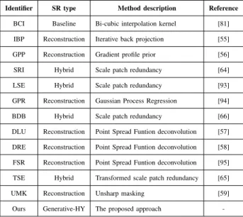
The performance of the proposed approach has been compared to the results obtained by 11 different un-supervised SR methods available in the literature, as well as the bi-cubic interpolation kernel function [81] used as a up-scaling baseline. These SR methods have been considered for the experimental discussion because of they provide an unsupervised SR scheme in the same way the proposed approach does, using the LR input image to generate a super-resolved output result. Additionally, two different scaling factors, 2× and4×, have been tested over the considered image dataset (Sec. A). Table III provides a brief description of the SR techniques considered in the experimental part of the work.
All the tested methods have been downloaded from the following website3 and they have been used con-sidering the default settings suggested by the methods’
3http://www.vision.uji.es/srtoolbox/
TABLE III
METHODS CONSIDERED FOR THE EXPERIMENTS. FURTHER DETAILS CAN BE FOUND IN THE CORRESPONDING REFERENCES.
Identifier SR type Method description Reference
BCI Baseline Bi-cubic interpolation kernel [81] IBP Reconstruction Iterative back projection [55] GPP Reconstruction Gradient profile prior [56]
SRI Hybrid Scale patch redundancy [64]
LSE Hybrid Scale patch redundancy [93]
GPR Reconstruction Gaussian Process Regression [94]
BDB Hybrid Scale patch redundancy [66]
DLU Reconstruction Point Spread Funtion deconvolution [57] DRE Reconstruction Point Spread Funtion deconvolution [58] FSR Reconstruction Point Spread Funtion deconvolution [95] TSE Hybrid Transformed scale patch redundancy [65]
UMK Reconstruction Unsharp masking [59]
Ours Generative-HY The proposed approach
-authors for each particular scaling ratio [54]. Note that this configuration provides the most general scenario to super-resolve a wide range of image types taking into account the tested image diversity.
B. Results
Tables V-VII present the quantitative assessment of the considered SR methods in terms of seven different quality metrics. Specifically, each table contains the super-resolved results of four test images and, for each image, the SR results are provided in rows consider-ing two different scalconsider-ing factors, 2× and 4×, which are shown in columns. Besides, Table IV provides the average results for the whole image collection in order to provide a global view.
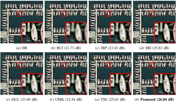
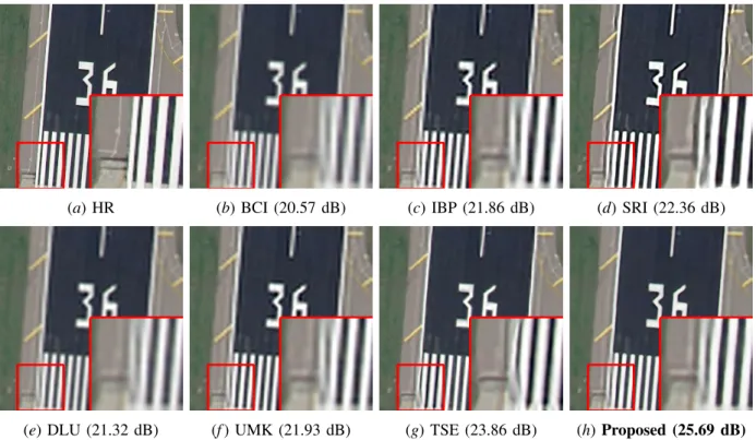
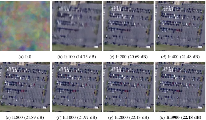
In addition to the quantitative evaluation provided by the considered metrics, some visual results are provided as a qualitative evaluation for the tested SR methods. Specifically, Figs. 6-7 show the super-resolved results obtained for harbor and road test images considering2× and 4× scaling factors, respectively. Besides, Fig. 8
TABLE IV
AVERAGESRRESULTS. THE BEST RESULT FOR SCALING RATIO AND METRIC IS HIGHLIGHTED IN BOLD FONT.
Image Method
Ratio 2x Ratio 4x
TIME NRMSE PSNR ERGAS Qindex SSIM SAM TIME NRMSE PSNR ERGAS Qindex SSIM SAM
Average BCI 0.01 0.0506 28.11 5.975 0.7915 0.8406 0.0160 0.01 0.0837 23.59 4.913 0.4769 0.6067 0.0233 IBP 0.15 0.0455 29.01 5.353 0.8200 0.8667 0.0174 0.48 0.0793 24.05 4.668 0.5474 0.6575 0.0260 GPP 25.30 0.0501 28.20 5.934 0.7870 0.8409 0.0178 17.46 0.0823 23.74 4.830 0.4847 0.6155 0.0244 SRI 337.77 0.0395 30.23 4.599 0.8337 0.8805 0.0167 335.30 0.0823 23.62 4.830 0.5490 0.6631 0.0272 LSE 1015.26 0.0510 27.83 5.874 0.7995 0.8546 0.0181 345.41 0.0865 23.15 4.925 0.5008 0.6454 0.0293 GPR 227.82 0.0693 25.29 8.179 0.6330 0.7215 0.0194 100.26 0.0888 23.03 5.202 0.4288 0.5734 0.0250 BDB 189.08 0.0904 22.80 10.660 0.6143 0.7093 0.0233 302.67 0.1341 19.26 7.873 0.2610 0.4569 0.0316 DLU 0.10 0.0458 28.96 5.374 0.8171 0.8642 0.0175 0.10 0.0811 23.87 4.767 0.4958 0.6220 0.0246 DRE 0.05 0.0458 28.96 5.374 0.8171 0.8642 0.0175 0.05 0.0811 23.87 4.767 0.4958 0.6220 0.0246 FSR 0.69 0.0575 26.85 6.825 0.7462 0.8170 0.0184 1.81 0.1015 21.81 5.974 0.2965 0.5190 0.0265 TSE 17.64 0.0397 30.18 4.626 0.8527 0.8902 0.0150 17.27 0.0742 24.73 4.386 0.5695 0.6820 0.0237 UMK 0.01 0.0457 28.97 5.367 0.8176 0.8647 0.0176 0.01 0.0789 24.11 4.648 0.5318 0.6465 0.0253 Ours 294.19 0.0376 30.57 4.366 0.8351 0.8836 0.0163 156.71 0.0704 25.21 4.193 0.5483 0.6776 0.0236
presents the visual evolution of the super-resolved result along the network iterations.
C. Discussion
According to the quantitative assessment reported in Tables V-IV, it is possible to rank the global performance of the tested SR methods into three different categories: (a) high performance: for the proposed approach, TSE and SRI, (b) moderate performance: for IBP, DLU, DRE and UMK, and (c) low performance: for GPP, LSE, GPR, BDB and FSR.
When considering a 2× scaling factor, the proposed approach (together with the hybrid methods TSE and SRI) provides a significant improvement with respect to the BCI baseline. Specifically, the proposed approach obtains the best performance for NRMSE, PSNR and ERGAS metrics, whereas TSE exhibits the best result for Q-index, SSIM and SAM. Although TSE and SRI also achieve, on average, a remarkable improvement over the baseline, the proposed approach provides a more consistent performance because it obtains the best average result for NRMSE, PSNR and ERGAS
met-rics, and the second best value for Q-index, SSIM and SAM. It can be observed that the average PSNR gain provided by the proposed approach is 0.39 dB for 2× and0.48dB for4×. Regarding the methods providing a moderate improvement (b), the PSF deconvolution-based techniques, DLU, DRE and UMK, provide a similar average performance and IBP is able to obtain a slightly better quantitative result over all the considered metrics. Within the low performance method group (c), it is possible to see that GPP and LSE methods provide a result similar to the one obtained by the baseline, and GPR, BDB and FSR obtain even a worse result.
A similar trend can be observed when considering a
4× scaling factor. In this case, the proposed approach is, on average, the best method according to NRMSE, PSNR and ERGAS metrics. TSE obtains the best Q-index and SSIM results, and both methods obtain a similar average result for the SAM metric. It should be noted that SRI performance has worsened when using a 4× ratio, however it still obtains the third best Q-index and SSIM results. With respect to the rest of the moderate (b) and low performance methods (c), they
(a) HR (b) BCI (21.73 dB) (c) IBP (23.43 dB) (d) SRI (25.82 dB)
(e) DLU (23.40 dB) (f) UMK (23.44 dB) (g) TSE (25.63 dB) (h) Proposed (26.84 dB)
Fig. 6. SR results obtained using the methods shown in captions over the test image harbor with a2×scaling factor. For each result, PSNR (dB) values appear in brackets. The best PSNR value is highlighted in bold.
obtain similar results with regards to the ones obtained with a 2× factor. Overall, the proposed approach and TSE have shown to obtain the best quantitative perfor-mance followed some way behind by SRI. However, the differences among these methods are relatively small, which motivates a thorough discussion over qualitative results to find out each method singularities.
According to the visual results presented in Figs. 6-7, each SR method tends to foster a particular kind of visual feature on the super-resolved output. Some methods, like TSE or SRI, are able to obtain sharper edges, while others, like DLU or UMK, seem more robust to noise by generating smoother super-resolved textures. In terms of visual perceived quality, the proposed approach achieves a remarkable performance. For instance, the boat detail in Fig. 6(h) is certainly the most similar to its HR coun-terpart in Fig. 6(a). Even though the result provided by SRI (Fig. 6(d)) seems to obtain a slightly better contrast
on some parts of the image, the proposed approach is able to introduce more high-frequency information in the boat structure. In addition, it is possible to see that the proposed approach also introduces some shadow fine details which are not present in the others methods’ results.
When considering a4×ratio, the proposed approach shows even better capability to recover high-frequency information while preserving HR details to avoid unde-sirable visual artifacts in the super-resolved output. For instance, it is the case of the result provided by SRI in Fig. 7(d) which provides a remarkable sharpness on edges, however it generates a kind of ghosting effect and also alters several shapes in the image. Despite the fact that TSE (Fig. 7(g)) is able to overcome some of these limitations, the proposed approach certainly provides a more competitive visual result. That is, the proposed approach generates a super-resolved image with sharper
(a) HR (b) BCI (20.57 dB) (c) IBP (21.86 dB) (d) SRI (22.36 dB)
(e) DLU (21.32 dB) (f) UMK (21.93 dB) (g) TSE (23.86 dB) (h) Proposed (25.69 dB)
Fig. 7. SR results obtained using the methods shown in captions over the test image road with a4×scaling factor. For each result, PSNR (dB) values appear in brackets. The best PSNR value is highlighted in bold.
edges and it is also able to reduce the aliasing effect present in the TSE result. Another illustrative difference can be found in the asphalt surface, where the proposed approach removes the noise appearing in other output results.
Regarding computational time, we can observe some important differences among the tested methods. In particular, three groups can be identified when super-resolving LR input images: (i) BCI, IBP, DLU, DRE, FSK and UMK, with an average time consumption per image under a second, (ii) GPP and TSE, with a time between 10 and 120 seconds, and (iii) the proposed approach, SRI, LSE, GPR and BDB which require more than 120 seconds per image. Even though the proposed approach is not one of the most computationally efficient methods, it shows a computational cost comparable to that of SRI which, on average, has shown to be among the best methods together with TSE and the proposed
approach.
D. Advantages and limitations of the proposed approach
When comparing the proposed approach performance with respect to the best ones obtained in the experiments, we can observe the high potential of the proposed deep generative network to super-resolve remote sensing data. To date, the hybrid approach used by SRI and TSE has shown to be one of the most effective ways to learn useful LR/HR patch relationships under an unsupervised SR scheme. However, this straightforward approach of searching patches across scales is rather constrained to the quality of the spatial information appearing in the LR input image. That is, the super-resolved result often tends to suffer from ghosting artifacts and watering effects as the magnification factor increases (Fig. 7).
Even though TSE deals with this issue by allowing patch geometric transformation on the searching patch
criteria, i.e. patches can occur in a lower scale as they are or even transformed, this process does not actually introduce any new spatial information in the output result which eventually may limit the SR process, especially in the remote sensing field. Note that remotely sensed imagery are usually a highly complex kind of data because they are usually fully-focused multi-band shots with plenty of different spatial details within the same image. As a result, the generation of a consistent spatial variability becomes a key factor to improve the unsupervised remote sensing SR process.
Precisely, this is the objective of the proposed ap-proach. In particular, the presented deep generative net-work learns the relationships between the LR and HR domains throughout several convolutional and down-sampling layers starting from the LR input image. How-ever, this process is affected by random noise which is also restricted by the cost function, i.e. equation (5), to guarantee a global reconstruction constraint over the LR input image. That is, the random noise generates new spatial variations as possible solutions to relieve the ill-posed nature of the SR problem, while the cost optimizer controls that only these variations consistent with respect to the input LR image are promoted though the network to generate the final SR result. Fig. 8 depicts the SR process conducted by the proposed network over the parking test image considering a 4× scaling factor. As we can see, the reconstructed super-resolved result is initially noise; however, the spatial structures are recovered from a coarser to finer level of details as the network iterates.
In a sense, the proposed approach is able to recover a richer variety of high-frequency patterns for a given LR image due to its generative nature. In other words, the proposed deep generative network provides a more flexible unsupervised SR scheme than the current hybrid techniques, because it is able to introduce some spatial
variations that are impossible to retrieve from the LR input image. In fact, it is possible to better appreciate the proposed approach effectiveness when only considering the PSNR metric, which is the most widely used quality index in SR. Figs. 9-10 show the PSNR gain obtained by the three best methods, i.e. the proposed approach, TSE and SRI, with respect to the BCI baseline. As we can appreciate, the proposed approach provides some remarkable PSNR improvements in 2×, however the PSNR gain is consistently higher when considering a
4× ratio. Note that, with this scaling factor, the level of uncertainty significantly increases and it is then when the generative process of the proposed approach becomes more effective by introducing a higher variety of spatial details.
Although the results obtained by the proposed ap-proach are encouraging, there are two points which deserve to be mentioned when comparing the proposed approach performance to the one obtained by the most effective unsupervised SR methods; the performance on some metrics and the computational cost.
On the one hand, the proposed approach performances on some metrics, specifically Q-index, SSIM and SAM, seem not to be superior than the corresponding TSE re-sults. For instance, Table VII shows that the TSE obtains the best SSIM result for the 4× road image (0.8290) whereas the proposed approach achieves the second best SSIM value (0.8247). However, the proposed approach provides the best PSNR result (25.69 dB) which is substantially higher than the TSE one (23.86 dB). In spite of the small SSIM differences, it is possible to see the proposed approach advantages when considering the qualitative results. That is, Fig. 10 certainly shows that TSE magnifies the aliasing effect in the fist line of pedestrian crossing and also generates a kind of watering effect on surfaces whereas the proposed approach is able to obtain a more natural as well as reliable result even
(a) It.0 (b) It.100 (14.73 dB) (c) It.200 (20.69 dB) (d) It.400 (21.48 dB)
(e) It.800 (21.89 dB) (f) It.1000 (21.97 dB) (g) It.2000 (22.13 dB) (h)It.3900 (22.18 dB)
Fig. 8. SR process conducted by the proposed approach over the parking test image with a4×scaling factor. Each sub-figure represents the obtainedXHR
o images at each epoch of the model, following Algorithm 1.
Fig. 9. PSNR (dB) results when considering a2×scaling factor.
though some image materials seem less contrasted. For the proposed approach, we adopt a cost function based on the mean-squared-error (MSE) in the way many other deep learning-based SR methods do in the supervised scheme, e.g. [69]–[71]. Logically, our model has a differ-ent nature because of its unsupervised scheme, however it seem reasonable to make this consideration because the PSNR index, which is based on the MSE, is one the most
Fig. 10. PSNR (dB) results when considering a4×scaling factor.
commonly used metric in SR. Somehow, this definition of the cost function may constrain the performance on some metrics because the network optimizer works for minimizing the MSE and other kinds of metric features are not taken into account in this optimization process, which eventually may led to a super-resolved solution with an excellent PSNR performance but with some small divergences in other figures of merit.
On the other hand, the computational cost of the proposed approach may also become a limitation in some specific scenarios. According to the quantitative results shown in Table IV, the proposed approach takes over 300 and 150 seconds to process each input image con-sidering a 2× and4×ratios respectively. Even though the proposed approach has shown not to be one of the most computationally efficient methods, three important considerations have to be done to this extent. First, the computational burden is not only a drawback of the proposed approach but also of any deep learning architecture because this kind of technology usually provides a more powerful framework to cope with new challenges and tasks. Second, the implementation of our model has not been optimized to really exploit the GPU hardware resources in order to substantially reduce the resulting computational time. That is, we make use of standard functions but further efforts could be addressed to generate a much more optimized version of the code. Third, we use a general configuration of
4,000 iterations as a security margin to guarantee a good network convergence, however this value could be reduced in order to significantly improve the proposed approach computational efficiency. Fig. 11 shows the evolution of the PSNR metric with respect to the number of iteration for harbor, circular-farmland, industry and road test images with a4×ratio. As it is possible to see, the network is able to achieve a PSNR result that is very close to the optimal value after 2,000 iterations, therefore it would be possible to reduce the number of iterations in order to significantly decrease the proposed approach computational time. In Fig. 12, we also show the PSNR evolution over time to highlight the fact that the proposed approach is able to rapidly converge to the optimal PSNR value. It should be noted that we use a unique network settings in this work, therefore4,000iterations are used to guarantee a good general parameter convergence, that
Fig. 11. PSNR evolution for harbor, circular-farmland, industry and road test images considering a4×scaling ratio versus iteration.
Fig. 12. PSNR evolution for harbor, circular-farmland, industry and road test images considering a4×scaling ratio versus time.
is, without adapting the network to each input image.
V. CONCLUSIONS ANDFUTURELINES
In this work, we have presented a new convolutional generator model to super-resolve LR remote sensing data from an unsupervised perspective. Specifically, the proposed approach is initially able to learn relationships between the LR and HR domains while generating con-sistent random spatial variations. Then, the data is sym-metrically projected to the target resolution, guaranteeing a reconstruction constraint over the LR input image. Our experiments, conducted using several test images, 2 scaling factors and 12 different SR methods available in the literature, reveal the competitive performance of the proposed approach when super-resolving remotely sensed images.
One of the main conclusions that arises from this work is the potential of deep generative models to cope with the unsupervised SR problem, because of their capabilities to introduce new spatial details not present in the input LR image. As opposed to the common (hybrid) SR trend, which only relies on the patch relationships learned across scales, the proposed approach extends this scheme by introducing some spatial variations that allow the network to retrieve new spatial patterns that are consistent with the input LR image.
According to the conducted experiments, the proposed approach obtains a competitive global performance over the considered remote sensing test images in terms of both quantitative and qualitative SR results. Regarding the NRMSE, PSNR and ERGAS metrics, the SR frame-work proposed in this frame-work obtains, on average, the best performance. When considering Q-index, SSIM and SAM, TSE tends to provide the best average result, but the proposed approach is still able to perform among the best methods, especially when considering a4×scaling factor.
Although the proposed approach results are encour-aging as a generative SR model in remote sensing, the method still has some limitations which provide room for improvement by conducting additional research on unsupervised SR. Specifically, our future work will be aimed at the following directions: (i) extending the cost function to simultaneously take into account several image quality metrics and also to extend it with the aim of implementing a noise reduction scheme for a different kind of input data, (ii) adapting the convolutional kernel size to each specific input image, and (iii) reducing the model computational cost by designing new strategies to actively control the number of iterations depending on the input image.
ACKNOWLEDGMENT
The authors would like to gratefully acknowledge the Editors and Reviewers for their outstanding comments and suggestions, which greatly helped us to improve the technical quality and presentation of this work.
REFERENCES
[1] J. A. Benediktsson, J. Chanussot, and W. M. Moon, “Very high-resolution remote sensing: Challenges and opportunities,” Proceedings of the IEEE, vol. 100, no. 6, pp. 1907–1910, 2012. [2] M. T. Pham, E. Aptoula, and S. Lefvre, “Feature profiles from attribute filtering for classification of remote sensing images,” IEEE Journal of Selected Topics in Applied Earth Observations and Remote Sensing, vol. 11, no. 1, pp. 249–256, 2018. [3] A. E. Maxwell, T. A. Warner, and F. Fang, “Implementation
of machine-learning classification in remote sensing: an applied review,”International Journal of Remote Sensing, vol. 39, no. 9, pp. 2784–2817, 2018.
[4] G. Sumbul, R. G. Cinbis, and S. Aksoy, “Fine-grained object recognition and zero-shot learning in remote sensing imagery,” IEEE Transactions on Geoscience and Remote Sensing, vol. 56, no. 2, pp. 770–779, 2018.
[5] X. Kang, Y. Huang, S. Li, H. Lin, and J. A. Benediktsson, “Extended random walker for shadow detection in very high reso-lution remote sensing images,”IEEE Transactions on Geoscience and Remote Sensing, vol. 56, no. 2, pp. 867–876, 2018. [6] H. Lin, Z. Shi, and Z. Zou, “Fully convolutional network with
task partitioning for inshore ship detection in optical remote sensing images,”IEEE Geoscience and Remote Sensing Letters, vol. 14, no. 10, pp. 1665–1669, 2017.
[7] T. Wu, J. Luo, J. Fang, J. Ma, and X. Song, “Unsupervised object-based change detection via a weibull mixture model-based binarization for high-resolution remote sensing images,” IEEE Geoscience and Remote Sensing Letters, vol. 15, no. 1, pp. 63– 67, 2018.
[8] Z. Liu, G. Li, G. Mercier, Y. He, and Q. Pan, “Change detec-tion in heterogenous remote sensing images via homogeneous pixel transformation,”IEEE Transactions on Image Processing, vol. 27, no. 4, pp. 1822–1834, 2018.
[9] A. S. Belward and J. O. Skøien, “Who launched what, when and why; trends in global land-cover observation capacity from civilian earth observation satellites,” ISPRS Journal of Pho-togrammetry and Remote Sensing, vol. 103, pp. 115–128, 2015. [10] T. S. Unger Holtz, “Introductory digital image processing: A
[11] S. C. Park, M. K. Park, and M. G. Kang, “Super-resolution image reconstruction: a technical overview,” IEEE signal processing magazine, vol. 20, no. 3, pp. 21–36, 2003.
[12] P. Milanfar,Super-resolution imaging. CRC press, 2010. [13] L. Yue, H. Shen, J. Li, Q. Yuan, H. Zhang, and L. Zhang, “Image
super-resolution: The techniques, applications, and future,”Signal Processing, vol. 128, pp. 389–408, 2016.
[14] A. Garzelli, “A review of image fusion algorithms based on the super-resolution paradigm,” Remote Sensing, vol. 8, no. 10, p. 797, 2016.
[15] C.-Y. Yang, C. Ma, and M.-H. Yang, “Single-image super-resolution: A benchmark,” inEuropean Conference on Computer Vision, 2014.
[16] A. Punnappurath, T. M. Nimisha, and A. N. Rajagopalan, “Multi-image blind super-resolution of 3d scenes,”IEEE Transactions on Image Processing, vol. 26, no. 11, pp. 5337–5352, 2017. [17] D. Yang, Z. Li, Y. Xia, and Z. Chen, “Remote sensing image
super-resolution: Challenges and approaches,” inDigital Signal Processing (DSP), 2015 IEEE International Conference on, 2015, pp. 196–200.
[18] L. Alparone, B. Aiazzi, S. Baronti, and A. Garzelli, Remote sensing image fusion. Crc Press, 2015.
[19] C. M. Bishop, Neural Networks for Pattern Recog-nition. Clarendon Press, 1995. [Online]. Available: https://books.google.es/books?id=-aAwQO -rXwC
[20] J. A. Benediktsson, P. H. Swain, and O. K. Ersoy, “Conjugate gradient neural networks in classification of very high dimensional remote sensing data,” International Journal of Remote Sensing, vol. 14, no. 15, pp. 2883–2903, 1993. [Online]. Available: http://www.tandfonline.com/doi/abs/10.1080/01431169308904316 [21] P. M. Atkinson and A. R. L. Tatnall, “Introduction Neural
networks in remote sensing,” International Journal of Remote Sensing, vol. 18, no. 4, pp. 699–709, 1997. [Online]. Available: http://dx.doi.org/10.1080/014311697218700
[22] H. Yang, “A back-propagation neural network for mineralogical mapping from AVIRIS data,” International Journal of Remote Sensing, vol. 20, no. 1, pp. 97–110, 1999. [Online]. Available: http://dx.doi.org/10.1080/014311699213622
[23] Y. LeCun, Y. Bengio, and G. Hinton, “Deep Learning,”Nature, vol. 521, p. 436444, 2015.
[24] I. Goodfellow, Y. Bengio, and A. Courville,Deep Learning. MIT Press, 2016.
[25] Y. Bengio, “Learning Deep Architectures for AI,” Machine Learning, vol. 2, no. 1, pp. 1–127, 2009.
[26] M. Sharma, S. Chaudhury, and B. Lall, “Deep learning based frameworks for image resolution and noise-resilient super-resolution,” in 2017 International Joint Conference on Neural Networks (IJCNN), May 2017, pp. 744–751.
[27] K. Makantasis, K. Karantzalos, A. Doulamis, and N. Doulamis, “Deep supervised learning for hyperspectral data classification through convolutional neural networks,” in 2015 IEEE Interna-tional Geoscience and Remote Sensing Symposium (IGARSS), 2015, pp. 4959–4962.
[28] M. Castelluccio, G. Poggi, C. Sansone, and L. Verdoliva, “Land use classification in remote sensing images by convolutional neural networks,” CoRR, vol. abs/1508.00092, 2015. [Online]. Available: http://arxiv.org/abs/1508.00092
[29] Y. Chen, H. Jiang, C. Li, X. Jia, and P. Ghamisi, “Deep Feature Extraction and Classification of Hyperspectral Images Based on Convolutional Neural Networks,” IEEE Transactions on Geoscience and Remote Sensing, vol. 54, no. 10, pp. 6232–6251, 2016. [Online]. Available: http://ieeexplore.ieee.org/document/7514991/
[30] M. E. Paoletti, J. M. Haut, J. Plaza, and A. Plaza, “A new deep convolutional neural network for fast hyperspectral image classification,” ISPRS Journal of Photogrammetry and Remote Sensing, 2017.
[31] Q. Yuan, Y. Wei, X. Meng, H. Shen, and L. Zhang, “A multiscale and multidepth convolutional neural network for remote sensing imagery pan-sharpening,” IEEE Journal of Selected Topics in Applied Earth Observations and Remote Sensing, 2018. [32] R. Dian, S. Li, A. Guo, and L. Fang, “Deep hyperspectral
image sharpening,”IEEE Transactions on Neural Networks and Learning Systems, 2018.
[33] Q. Zhang, Q. Yuan, C. Zeng, X. Li, and Y. Wei, “Missing data reconstruction in remote sensing image with a unified spatial-temporal-spectral deep convolutional neural network,” IEEE Transactions on Geoscience and Remote Sensing, 2018. [34] L. Liebel and M. Krner, “Single-image super resolution for
multispectral remote sensing data using convolutional neural networks,” vol. XLI-B3, pp. 883–890, 06 2016.
[35] C. Dong, C. C. Loy, K. He, and X. Tang, “Image super-resolution using deep convolutional networks,”IEEE Transactions on Pat-tern Analysis and Machine Intelligence, vol. 38, no. 2, pp. 295– 307, Feb 2016.
[36] T. Y. Han, Y. J. Kim, and B. C. Song, “Convolutional neural network-based infrared image super resolution under low light environment,” in2017 25th European Signal Processing Confer-ence (EUSIPCO), Aug 2017, pp. 803–807.
[37] C. Li, Z. Ren, B. Yang, X. Wan, and J. Wang, “Texture-centralized deep convolutional neural network for single image super resolution,” in2017 Chinese Automation Congress (CAC), Oct 2017, pp. 3707–3710.
[38] X. Du, Y. He, J. Li, and X. Xie, “Single image super-resolution via multi-scale fusion convolutional neural network,” in 2017 IEEE 8th International Conference on Awareness Science and Technology (iCAST), Nov 2017, pp. 544–551.