Approaches to Feature Identification and Feature Selection for Binary and Multi-Class Classification

(1)

Approaches to Feature Identiﬁcation and Feature

Selection for Binary and Multi-Class Classiﬁcation

A DISSERTATION

SUBMITTED TO THE FACULTY OF THE GRADUATE SCHOOL OF THE UNIVERSITY OF MINNESOTA

BY

Zisheng Zhang

IN PARTIAL FULFILLMENT OF THE REQUIREMENTS FOR THE DEGREE OF

Doctor of Philosophy

KESHAB K. PARHI

(2)

c

(3)

Acknowledgments

I would like to express my sincere gratitude to my advisor Professor Keshab K. Parhi for his utmost support and guidance throughout the years of my graduate study. It is my greatest pleasure to have Dr. Parhi as my academic teacher, research mentor, and spiritual guide. Those tremendous time that we spent together on brain storming, paper writing, problem solving will be my most precious memories forever. His motivation, enthusiasm, immense knowledge and commitment to excellence has always inspired me to be a better researcher and a better person.

I am extremely fortunate to have the opportunity to work with Dr. Thomas R. Henry, Dr. Zhiyi Sha, and Dr. Tay Netoﬀ for the past three to four years. Their patience, immense knowledge, and great commitment have made our collaboration pos-sible. Their insightful comments, suggestions, and support have made our joint work successful. I am truly thankful to them.

I owe sincere thankfulness to Professor Mostafa Kaveh, Emad Ebbini, and Tay Netoﬀ for serving on my defense committee. I have beneﬁted from interacting with them and learned the knowledge that I need for completing my graduate study. I am very grateful to have my labmates and friends: Dr. Yingjie Lao, Dr. Tingting Xu, Dr. Bo Yuan, Dr. Yun Sang Park, Yin Liu, Shu-Hsien (Dennis) CHU, and many other friends who have helped me. They have made my graduate study at UMN meaningful and colorful. It has been the greatest privilege to have my Chinese friends and buddies: Wei Zhang, Keping Song, Yinglong Feng, Yi Wang, Xiaofan Wu, Jie Kang, Yu Chen, Jun Fang, Cong Ma, Kejian Wu, and many others. They have become an important part of my life in Minnesota. I will always remember the great times we have spent together.

I would like to sincerely thank my host family, Peter Michel. He helped me settle down when I ﬁrst came the United States and taught me many traditions in this country.

(4)

at Leanics Corporation. A patent on this topic was ﬁled by Prof. Keshab Parhi, Leanics owner.

Last but not lest, I would like to sincerely thank my family. My parents have always been teaching me to study hard, work hard, party hard and enjoy life. They always encourage me and cheer me up when I am down. They always guide me through diﬃcult time and help me pursue my dreams. Without their unconditional support, I would not be the person I am today.

(5)

Abstract

In this dissertation, we address issues of (a) feature identiﬁcation and extraction, and (b) feature selection. Nowadays, datasets are getting larger and larger, especially due to the growth of the internet data and bio-informatics. Thus, applying feature extraction and selection to reduce the dimensionality of the data size is crucial to data mining.

Our ﬁrst objective is to identify discriminative patterns in time series datasets. Using auto-regressive modeling, we show that, if two bands are selected appropriately, then the ratio of band power is ampliﬁed for one of the two states. We introduce a novel

frequency-domain power ratio(FDPR) test to determine how these two bands should be selected. The FDPR computes the ratio of the two model filter transfer functions where the model filters are estimated using different parts of the time-series that correspond to two different states. The ratio implicitly cancels the effect of change of variance of the white noise that is input to the model. Thus, even in a highly non-stationary environment, the ratio feature is able to correctly identify a change of state. Synthesized data and application examples from seizure prediction are used to prove validity of the proposed approach. We also illustrate that combining the spectral power ratios features with absolute spectral powers and relative spectral powers as a feature set and then carefully selecting a small number features from a few electrodes can achieve a good detection and prediction performances on short-term datasets and long-term fragmented datasets collected from subjects with epilepsy.

Our second objective is to develop efficient feature selection methods for binary clas-sification (MUSE) and multi-class clasclas-sification (M3U) that effectively select important features to achieve a good classification performance. We propose a novel incremental feature selection method based on minimum uncertainty and feature sample elimination (referred as MUSE) for binary classification. The proposed approach differs from prior mRMR approach in how the redundancy of the current feature with previously selected features is reduced. In the proposed approach, the feature samples are divided into a pre-specified number of bins; this step is referred to as feature quantization. A novel

uncertainty score for each feature is computed by summing the conditional entropies of the bins, and the feature with the lowest uncertainty score is selected. For each bin, its

(6)

2. The feature samples corresponding to the bins with impurities below a threshold are discarded and are not used for selection of the subsequent features. The signiﬁcance of the MUSE feature selection method is demonstrated using the two datasets: arrhythmia and hand digit recognition (Gisette), and datasets for seizure prediction from ﬁve dogs and two humans. It is shown that the proposed method outperforms the prior mRMR feature selection method for most cases.

We further extends the MUSE algorithm for multi-class classification problems. We propose a novel multiclass feature selection algorithm based on weighted conditional entropy, also referred to as uncertainty. The goal of the proposed algorithm is to select a feature subset such that, for each feature sample, there exists a feature that has a low uncertainty score in the selected feature subset. Features are firstquantized into different bins. The proposed feature selection method first computes an uncertainty vector from

weighted conditional entropy. Lower the uncertainty score for a class, better is the separability of the samples in that class. Next, an iterative feature selection method selects a feature in each iteration by (1) computing the minimum uncertainty score for each feature sample for all possible feature subset candidates, (2) computing the average minimum uncertainty score across all feature samples, and (3) selecting the feature that achieves the minimum of the mean of the minimum uncertainty score. The experimental results show that the proposed algorithm outperforms mRMR and achieves lower misclassification rates using various types of publicly available datasets. In most cases, the number of features necessary for a specified misclassification error is less than that required by traditional methods.

(7)

List of Tables

2.1 Detection Performance of The System using linear SVM . . . 24 2.2 Detection Performance of The System using Adaboost . . . 25 2.3 Comparison to prior work . . . 26 3.1 Prediction Performance of The Proposed System using a single feature

for MIT Database . . . 49 4.1 Detection Performance of The Proposed System . . . 57 4.2 Comparison to prior work . . . 59 5.1 Prediction Performance of The Proposed System using a single feature

for Freiburg Database . . . 75 5.2 Prediction Performance of The Proposed System using a single feature

for MIT Database . . . 76 5.3 Prediction Performance of The Proposed System using BAB for Freiburg

Database . . . 76 5.4 Prediction Performance of The Proposed System using BAB for MIT

Database . . . 77 5.5 Overall Prediction Performance of The Proposed System for Freiburg and

MIT Databses . . . 77 5.6 Comparison of Prediction Performance between BAB and LASSO for

Freiburg Database . . . 78 5.7 Comparison of Prediction Performance between BAB and LASSO for

MIT Database . . . 78 5.8 Synthesis Results Of 1024-Point Serial Rﬀt For 100 MHz Clock Frequency 80 5.9 Comparison of Energy Consumption between Linear SVM and RBF-SVM

for MIT Database. . . 82

(13)

5.10 Comparison to prior work . . . 83 6.1 Comparing the Prediction Performance of The System using RBF-SVM

and the proposed method with Polynomial-SVM . . . 94 6.2 Comparison of Prediction Performance using Diﬀerent Feature Sets and

Classiﬁers on the Testing Dataset . . . 94 6.3 Best Prediction Performance on Testing Data . . . 95 7.1 Conditional Entropy for mRMR and the Proposed Method and its

Esti-mated Value. . . 110 7.2 Description of Arrhythmia and Gisette datasets. . . 116 7.3 Seizure Prediction Dataset from Kaggle Contest. . . 117 7.4 Classiﬁcation Performance on the American Epilepsy Society Seizure

Pre-diction Challenge database Using CART . . . 120 7.5 Classiﬁcation Performance on the American Epilepsy Society Seizure

Pre-diction Challenge database Using ANN . . . 123 8.1 An Example For A Quantized Feature With 5 Bins And 4 Classes. . . . 134 8.2 Entropy With Weighting For The Features Shown in Table 8.1. . . 134 8.3 Entropy Without Weighting For The Features Shown in Table 8.1. . . . 134 8.4 Coding Example for a 3-class OVO multclass classiﬁcation. . . 138 8.5 Description of The Four Datasets. . . 140 8.6 Misclassiﬁcation Rate for the Proposed Algorithm and mRMR for the

Smartphone-Based Recognition of Human Activities and Postural Tran-sitions Data Set using Decision Tree. . . 142 8.7 Misclassiﬁcation Rate for the Proposed Algorithm and mRMR for the

Sensorless Drive Diagnosis Data Set using Decision Tree. . . 144 8.8 Misclassiﬁcation Rate for the Proposed Algorithm and mRMR for the

Otto Group Product Dataset using Decision Tree. . . 145 8.9 Misclassiﬁcation Rate for the Proposed Algorithm and mRMR for the

Forest Type Prediction Dataset using Decision Tree. . . 145

(14)

List of Figures

1.1 General framework for machine learning. . . 2

1.2 Mean power of the whitened EEG signal from electrode No. 1 for patient No. 19 in the MIT physionet EEG database. . . 4

1.3 Structure of a 2-level wavelet decomposition . . . 7

2.1 System architecture for seizure detection . . . 20

2.2 Percentage of total energy captured by the predictor versus the predic-tor’s order using (a) an hour’s inter-ictal data from patient No. 1 while the patient is awake and (b) an hour’s inter-ictal data from patient No. 1 while the patient is sleeping. . . 22

2.3 Spectrograms of the EEG signal (left) and its error signal (right) using interictal recordings for the 16th hour from patient No. 1. . . 22

2.4 Feature extraction. . . 23

3.1 System models at (a) State 1 and (b) State 2. . . 29

3.2 magnitudes of frequency responses for the system in two states. . . 29

3.3 Histogram of the logarithm of the band power in the frequency band of [0,0.2π] for segments of x1 and x2.. . . 31

3.4 Histogram of the band powers in (a) frequency band of [0,0.2π], and in (b) frequency band of [0.3π,0.4π]. . . 32

3.5 Magnitude of the ratio betweenH1andH2, i.e.,|H2(ejω)|/|H1(ejω)|from 0 to 0.4π. . . 35

3.6 Histogram of the ratio between the band powers in frequency band of [0,0.2π], and the band power in the frequency band of [0.2π,0.4π]. . . . 36

3.7 PEF for the system at (a) State 1, and (b) State 2. . . 36

3.8 Auto-regressive models for (a)x1, and (b)x2. . . 37

(15)

3.9 Magnitude of the AR(19) PEF for the synthesized signals in State 1 and State 2. . . 39 3.10 RH(ejω) versus frequencyω, where the blue horizontal line represents the

baseline. . . 39 3.11 (a) Spectral power ratio between the band power in the frequency band

of [0.8π, π] and the band power in the frequency band of [0,0.1π] for each segment and (b) the input noise variance for each segment. . . 40 3.12 Histogram of (a) the band power in the frequency band of [0.8π, π], (b) the

band power in the frequency band of [0,0.1π], and (c) the ratio between the above 2 band powers. . . 41 3.13 Scatter plot of the logarithm of the band power in the frequency band of

[0.8π, π] and the logarithm of the band power in the frequency band of [0,0.1π] for each segment in 2 states. . . 41 3.14 AUC versus the SNR in dB scale for the band power in the frequency

band of [0.8π, π], the band power in the frequency band of [0,0.1π], and their ratio.. . . 42 3.15 The same spectral power ratio between the band power in the frequency

band of [0.8π, π] and the band power in the frequency band of [0,0.1π] as shown in Fig. 3.11 for State 1 and State 2 before and after post-processing in a low-SNR case, where SNR=2dB. . . 43 3.16 AUC versus the SNR in dB scale for the band power in the frequency

band of [0.8π, π], the band power in the frequency band of [0,0.1π], and their ratio after Kalman ﬁlter. . . 44 3.17 AUC versus the SNR in dB scale for diﬀerent choices of frequency bands. 44 3.18 The magnitude of the ratio between the frequency response of the PEF

for preictal signal and the frequency response of the PEF for the interictal signal in electrode No. 17 for Patient No. 1. . . 46 3.19 The magnitude of the ratio between the frequency response of the PEF

for preictal signal and the frequency response of the PEF for the interictal signal in electrode No. 20 for Patient No. 8. . . 46

(16)

for preictal signal and the frequency response of the PEF for the interictal signal in electrode No. 1 for Patient No. 21. . . 47 3.25 Band power in γ2 band (top pannel), band power in γ3 band (middle

pannel) and the spectral power ratio ofγ2−to−γ3 after Kalman ﬁlter using the EEG recordings in electrode No. 1 of Patient No. 19 in the MIT Physionet database. . . 48 4.1 Flow chart of the proposed algorithm for seizure detection . . . 53 4.2 Spectral power in in band [13,30] Hz (top pannel), spectral power in

band [160,200] Hz (middle pannel) and the spectral power ratio ofP8,13

-to-P160,200 using the EEG recordings in electrode No. 10 of patient No.

8 from the Upenn and Mayo Clinic’s database. . . 54 4.3 A three-node regression tree for patient No. 7 from the Upenn and Mayo

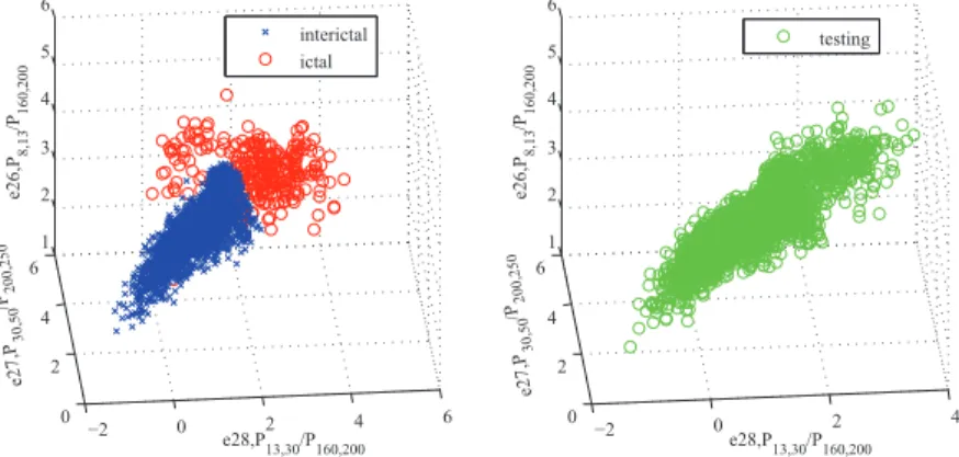
Clinic’s seizure detection contest. . . 55 4.4 3D scatter plot of the interictal and ictal feature vectors (left pannel) and

the 3D scatter plot of the testing feature vectors after feature selection by CART using the EEG recordings Patient No. 7 from the Upenn and Mayo Clinic’s database. . . 55 4.5 Conversion form decision variable to seizure probability for Pat. No. 8. 56

(17)

4.6 Relationship between detection horizon and speciﬁcity at diﬀerent thresh-olds. . . 58 5.1 Spectral power inγ2 band (top pannel), spectral power inγ1 band

(mid-dle pannel) and the spectral power ratio ofγ2-to-γ1 after postprcossing using the EEG recordings in electrode No. 1 of Patient No. 19 in the MIT Physionet database. . . 63 5.2 Flow chart of single feature selection. . . 64 5.3 Examples to illustrate the single ratio feature selected for seizure

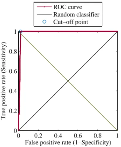
predi-tion and the power of the Kalman ﬁlter using the (a) ictal and (b) inter-ictal recordings from Patient No. 1 in the Freiburg database. . . 66 5.4 ROC analysis using Patient No. 1’s feature signal from the MIT EEG

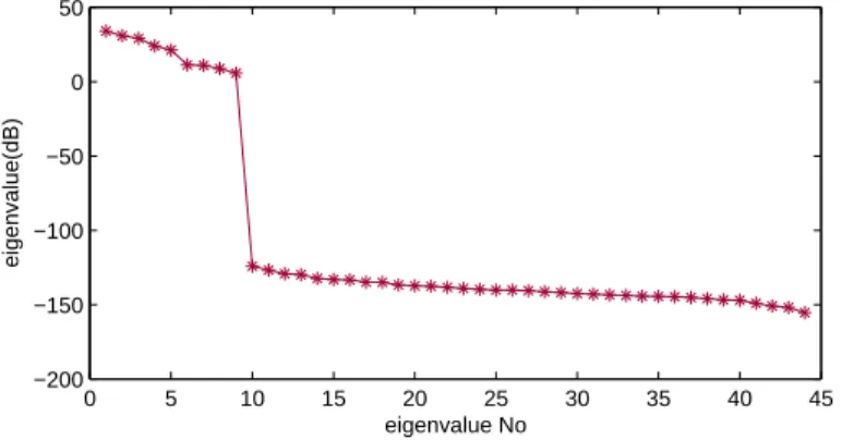
database. . . 67 5.5 Flow chart of single feature selection. . . 68 5.6 Eigenvalues of the covariance matrix of the features using Patient No.

14’s data from the MIT sEEG database.) . . . 69 5.7 Linear separability criteriaJ of the subset of features with diﬀerent

fea-ture dimensions using Patient No. 14’s recordings in electrode No. 14 from the MIT database. . . 72 5.8 Comparison the feature selection results of (a) LASSO and (b) BAB for

Patient No. 15 in the Freiburg database. . . 74 5.9 System architecture for PSD estimation. . . 79 5.10 Fully real serial FFT architecture. . . 80 5.11 System architectures for extracting (a) a single absolute spectral in a

specific band, (b) a relative spectral power in a specific band, and (c) a ratio of spectral powers in two bands from the PSD coefficients. . . 81 5.12 System architecture for linear SVM. . . 82 6.1 Flow chart of the proposed algorithm for seizure prediction . . . 87 6.2 Spectral power in in band [8,13] Hz (top pannel), spectral power in band

[13,30] Hz (middle pannel) and the spectral power ratio ofP8,13-to-P13,30

using the EEG recordings in electrode No. 13 of Patient No. 1 from the American Epilepsy Society Seizure Prediction Challenge database. . . . 89

(18)

10 using the EEG recordings of Patient No. 2 from the American Epilepsy Society Seizure Prediction Challenge database. . . 90 6.4 A three-node regression tree for Patient No. 1 from the American

Epilep-sy Society Seizure Prediction Challenge database. . . 91 6.5 Feature importance and electrode importance for Dog No. 1 from the

American Epilepsy Society Seizure Prediction Challenge database. . . . 91 6.6 Sorted feature importance for Dog No. 1 from the American Epilepsy

Society Seizure Prediction Challenge database in a descending order. . . 92 6.7 Conversion form decision variable to seizure probability for Dog. No. 1. 93 7.1 Histograms of (a) the original feature No. 939 and (b) quantized feature

No. 939 for Patient No. 1 in the American Seizure Prediction Challenge database. The details of this dataset are described in Section 7.4. . . 99 7.2 Flow chart of the proposed algorithm. . . 100 7.3 Proposed criteria (score) for each feature for the Gisette dataset. . . 103 7.4 Stacked histogram of the feature samples for Class 1 and Class 2 selected

by the proposed criterion for the Gisette dataset. . . 103 7.5 Bin impurities for the feature selected by the proposed criterion for the

Gisette dataset. . . 104 7.6 Bin impurities of the feature selected by the proposed criterion for Patient

No. 1 in the American Seizure Prediction Challenge database. . . 105 7.7 Stacked histogram of the feature samples for Class 1 and Class 2 selected

by the proposed algorithm (withp= 0.2) in the second iteration for the Gisette dataset. . . 106 7.8 Histograms of (a) feature No. 3 and (b) quantized feature No. 3 selected

in the second iteration with sample elimination using Dog No. 1 in the American Seizure Prediction Challenge database. . . 106 7.9 Histograms of the original feature No. 3 without sample elimination. . . 107 7.10 Flow chart of the proposed iterative feature sample elimination process. 108 7.11 Scatter plot of interictal features (blue crosses) and preictal features (red

circles) using the features selected by the proposed algorithm for Patient No. 1 in the American Seizure Prediction Challenge dataset. . . 111

(19)

7.12 Classification error rate of the Arrhythmia dataset for different quanti-zation levels using (a) Naive Bayes classifier, (b) LDA classifier, and (c)

CART classiﬁer. . . 113

7.13 Percentage of feature samples that survive for Class 1 and Class 2, re-spectively, after each iteration using the Gisette dataset, where the black dashed horizontal line represents the stopping threshold (Ts = 0.1 in this case). . . 114

7.14 Percentage of feature samples that survive for Class 1 (interictal) and Class 2 (preictal), respectively, after each iteration for Patient No. 1 in the American Seizure Prediction Challenge database. . . 115

7.15 Sensitivity (left panel) and specificity (right panel) for the Arrhythmia dataset from UCI for the proposed algorithm and mRMR using (a )Naive Bayes classifier, (b) LDA classifier, and (c) CART classifier. . . 119

7.16 Classification accuracies for Class 1 (left) and Class 2 (right) for the Gisette dataset from UCI between the proposed algorithm and mRMR using (a )Naive Bayes classifier, (b) LDA classifier, and (c) CART classifier.121 7.17 Comparison of (a) AUC, (b) sensitivity, and (c) specificity, for proposed algorithm and mRMR for the American Epilepsy Society Seizure Predic-tion Challenge database when CART is used. . . 123

7.18 Comparison of (a) AUC, (b) sensitivity, and (c) speciﬁcity, for proposed algorithm and mRMR for the American Epilepsy Society Seizure Predic-tion Challenge database when ANN is used. . . 125

8.1 A typical ﬂow chart for machine learning. . . 128

8.2 Flow chart for the proposed feature selection algorithms. . . 129

8.3 Block diagram for computing the proposed uncertainty vector. . . 130

8.4 Binary entropy. . . 132

8.5 Binary entropy. . . 133

8.6 An example for the proposed iterative feature selection algorithm. . . . 136 8.7 Classiﬁcation error rate versus No. of features for the Otto Group

Prod-uct Dataset using mRMR, proposed algorithm with weighted conditional entropy, and proposed algorithm with conventional conditional entropy. 141

(20)

Recognition of Human Activities and Postural Transitions Data Set using (a) SVM and (b) decision tree. . . 142 8.9 Classiﬁcation error rate versus No. of features for the Sensorless Drive

Diagnosis Data Set using (a) SVM and (b) decision tree. . . 143 8.10 Classiﬁcation error rate versus No. of features for the Otto Group

Prod-uct Dataset using (a) SVM and (b) decision tree. . . 144 8.11 Classiﬁcation error rate versus No. of features for the Forest Type

Pre-diction Dataset using decision tree. . . 145

(21)

Chapter 1

Introduction

1.1 Motivation

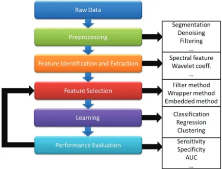
This dissertation addresses issues of (a) feature identification and extraction, and (b) feature selection. Data mining has been widely used in many areas, such as decision making, marketing, artificial intelligence, pattern recognition, and financial forecasts [1, 2, 3]. Fig. 1.1 illustrates a general framework for machine learning, which includes preprocessing, feature identification and extraction, feature selection, learning, and per-formance evaluation. Nowadays, datasets are getting larger and larger, especially due to the growth of the internet data and bio-informatics. However, high dimensionality of data may cause the curse of dimensionality problem [4, 5, 6]. Thus, applying feature extraction and selection to reduce the dimensionality of the data size is a crucial step in data mining.

Feature Identiﬁcation and Extraction

The problem of ﬁnding discriminative patterns in time series datasets has received much attention in past decades [7, 8, 9]. Time series are collected in a variety of applications such as electrocardiogram (ECG) [10, 11], electroencephalogram (EEG) [12, 13], hourly temperature and humidity [14], lung sounds [15], and stock prices [16], etc. A time series usually contains a lot of redundancy between consecutive samples as these samples are typically highly correlated. Feature extraction can be applied to extract discriminative features to extract useful information from the original signal and to reduce the data

(22)

Figure 1.1: General framework for machine learning.

size. The discriminative features can be input to classiﬁers to identify state of the time series.

In a typical pattern recognition problem for time series, we are faced with classifying the time series into different states. For instance, seizure prediction using EEG signals can be viewed as a binary classification problem where one class consists of preictal signals corresponding to the signal right before an occurrence of the seizure, and the other class consists of normal EEG signals, also referred as interictal signals [17, 18, 19, 20, 21]. Identifying features that can differentiate or discriminate the preictal state (time period before a seizure) from the inter-ictal state (time period between seizures) is the key to seizure prediction [22, 23, 24, 25, 26, 27, 28]. In a related but different problem of seizure detection, the EEG signal is classified into ictal (during seizure) and inter-ictal (baseline) [29, 30, 31]. In another example of the arrhythmia detection from ECG signals [32, 33], the aim is to distinguish between the presence and absence of cardiac arrhythmia. As another example, consider the Sensorless Drive Diagnosis problem [34, 35] using electric current drive signals. The drive has intact and defective components. This results in 11 different classes with different conditions. Each condition

(23)

3 has been measured several times by 12 diﬀerent operating conditions such as diﬀerent speeds, load moments and load forces. The current signals are measured with a current probe and an oscilloscope on two phases. The time series corresponding to the current signals are analyzed to classify whether a component is intact or defective. In another example, signals from the magnetoencephalogram (MEG) can be used to discriminate schizophrenia [36]. Seismograms also correspond to time-series that can be used to predict earthquakes.

Feature Selection

In the feature subset selection problem, a learning algorithm is faced with the problem of selecting a subset of features upon which to focus its attention, while ignoring the rest [37, 38, 39, 40]. Feature selection is the process of selecting a subset of relevant fea-tures for model construction. In contrast to other dimensionality reduction techniques like projection (e.g., principal component analysis) or compression (e.g., information theory), feature selection techniques do not change the original representations of the variables, but merely select a subset of them [41, 42]. Thus, they preserve the original meanings of the variables, oﬀering explanations for the data and the models.

While feature selection can be applied to both supervised and unsupervised learning, we focus here on the problem of supervised learning (classification), where the class labels are known beforehand [43, 44, 45]. The importance of feature selection techniques are manyfold which include: (1) avoid overfitting, (2) reduce time consumption of model training, (3) reduce energy consumptions in devices providing real-time classifications, and (4) simplify interpretations of different models [46].

1.2 Prior Works

This section reviews the prior works on feature identiﬁcation, feature selection, and classiﬁcation.

1.2.1 Prior Works on Feature Identiﬁcation and Extraction

Popular feature extraction techniques for time series include the discrete wavelet trans-form (DWT) [26], the discrete Fourier transtrans-form (DFT) [47], power spectral density

(24)

(PSD) [22, 23, 24], empirical mode decomposition (EMD) [48], eigenvectors [49], au-toregressive models [50], statistical values [51], instantaneous amplitude, frequency, or phase [52].

However, these features may not achieve a good classification performance for non-stationary signals. For instance, in the problem of seizure prediction, the preictal and interictal patterns vary substantially over different patients. Even for a single patient, preictal and interictal patterns may vary substantially from seizure to seizure and from hour to hour. For example, Fig. 1.2 illustrates the mean power of the whitened EEG signal from electrode No. 1 for patient No. 19 in the MIT physionet EEG database [53, 54], where a 10 second sliding window with no overlap is used. The EEG signal from electrode No. 1 is divided into 10-seconds-long segments and is then whitened for each segment. The variance of the whitened signal in each segment is computed as the mean power. As shown in the figure, the signal is very non-stationary as the variance of whitened signal changes significantly during the whole 29 hours. Mean power of the whitened signal during interictal period sometimes can be significantly higher than that of preictal signals. Therefore, extracting discriminative features from this signal to separate the preictal signal (60 minutes data prior to the seizure onsets) and the interictal signal is very challenging.

time(hour) 0 5 10 15 20 25 30 mean power 0 1000 2000 3000 4000

whitened signal power seizures onsets

Figure 1.2: Mean power of the whitened EEG signal from electrode No. 1 for patient No. 19 in the MIT physionet EEG database.

Window-based Signal Processing

Before feature extraction, the input signal,s(n), is divided into the input segments and the signal is processed segment by segment. Let M denote the length of each segment

(25)

5 and L denote the total number of segments. Let

sl(n) =s(n+ (l−1)M/2) (1.1) n= 0, . . . , M−1, l= 1, . . . , L (1.2) denote the windowed signal in the l-th segment. Each segment has a 50% overlap with its neighbour segment. Features can then be extracted from each segment.

Absolute spectral power

Absolute spectral power in a particular frequency band represents the power of a signal in that frequency band. To compute the (absolute) spectral powers in the above eight frequency bands, PSD of the input signal needs to be estimated. The PSD of a signal

s(n) describes the distribution of the signal’s total average power over frequency. The spectral power of a signal in a frequency band is computed as the logarithm of the sum of the PSD coeﬃcients within that frequency band. Mathematically, the spectral power in the i-th frequency band is computed as

Pi = log

∑

ω∈band i

P SDs(ω), i= 1,2, ...,8. (1.3)

For window-based signal processing, spectral power needs to be computed for each windowed segment sl(n):

Pi(l) = log

∑

ω∈band i

P SDsl(ω), i= 1,2, ...,8. (1.4)

Therefore, Pi(l) is a time series whose l-th element represents the spectral power of the

input signal in the l-th segment in band i.

Relative spectral power

The relative spectral power measures the ratio of the total power in the i-th band to the total power of the signal in logarithm scale, which is computed as follows

Qi(l) = log ∑ ω∈band i P SDsl(ω) ∑ all ω P SDsl(ω) , i= 1,2, ...,8. (1.5)

(26)

Spectral power ratio

Let Ri,j(l) = Pi(l)−Pj(l) represent the spectral power ratio of the spectral power in

bandiover that in bandjin thel-th window. These ratios indicate the change of power distribution in frequency domain from interictal to preictal periods, which have been shown in [30] to be good features for seizure detection and can also be used to predict seizures [55].

Cross-correlation coeﬃcients

Cross-correlation is a measure of similarity of two time series. Let si,l(n) and sj,l(n)

denote thel-th segments from thei-th electrode and from thej-th electrode respectively. The correlation coeﬃcient between the two segments is computed as follows:

ρi,j(l) =

∑

ninl-th segment

si,l(n)sj,l(n) (1.6)

Discrete wavelet decomposition

The purpose of wavelet decomposition is to decompose the original signal into three dis-joint sub-bands [56]. Discrete wavelet transform (DWT) decomposes discrete sequences into discrete wavelets coefficients. The structure of a 2-level wavelet decomposition tree is shown in Fig. 1.3. The input signal is first passed through a low-pass (LPF) and a high-pass (HPF) filter. Then each filter is followed by a down-sampler with factor of 2. At the next level, the approximation coefficients are further decomposed into approximate and detail coefficients.

1.2.2 Prior Works on Feature Selection

Feature selection techniques, in general, can be organized into three categories: ﬁlter methods, wrapper methods and embedded methods.

Filter feature selection methods apply a statistical measure to assign a score to each feature. The features are ranked by the score and then selected to be either kept or removed from the feature set. These methods are often univariate and consider each feature independently [38, 57].

(27)

7 1 2 2 Low-pass h(n) e(n) High-pass g(n) Ę2 a (n) Low-pass h(n) High-pass g(n) Ę2 Ę2 Ę2 d (n) d (n) e(n)

Figure 1.3: Structure of a 2-level wavelet decomposition

In a typical ﬁlter method, features can be ranked according to various means such as Fisher score [58],f-information[59], Bayes Error [60], Kolmogorov-Smirnov test [61], Pearson correlation [62], mutual information [63], Gini index [64], dependency [65], Henze-Penrose divergence [66], and consistency [44, 67]. Selection based on such a ranking method does not ensure weak dependency among features, and often can lead to redundancy and thus a less informative feature subset.

Wrapper methods consider the selection of a set of features as a search problem, where diﬀerent combinations are obtained, evaluated and compared to other combina-tions [68, 69, 70]. A predictive model is trained to evaluate each combination of features and assign a score based on model accuracy or other scores. As wrapper methods train a new model for each subset, they are very computationally intensive [68, 69].

The subset search process may include a methodical process such as best-ﬁrst search or branch and bound search [62, 71], stochastic optimization approaches such as a random hill-climbing algorithm, and heuristics approaches such as sequential forward and sequential backward selection (SFS and SBS) to add and remove features [72, 73]. Embedded methods identify which features best contribute to the accuracy of the model after the model is trained [74, 75, 76, 77]. The most common type of embedded feature selection methods are regularization methods.

Regularization methods are also called penalization methods that introduce addi-tional constraints into the optimization of a predictive algorithm (such as a regression algorithm) that bias the model toward lower complexity (less coeﬃcients).

(28)

For example, features can be selected using a tree classiﬁer and a model can then be trained on the selected features [29, 81]. In LASSO, a penalty term is added to the mean squared error to reduce the number features selected while minimizing the regression error. The drawbacks of such a method are its computational cost and sensitivity to overﬁtting.

Approaches of information-theoretic feature selection in machine learning have ad-vanced a lot over the past 15-20 years. Well-known criteria for feature selection include (1) Mutual Information Based Feature Selection (MIFS) [82], (2) Maximum-Relevance Minimum-Redundancy (mRMR) [83], (3) Joint Mutual Information (JMI) [84], (4) MIFS-U [85], (5) Conditional Infomax Feature Extraction (CIFE) [86], (6) Conditional Mutual Information Maximization (CMIM) [87], and (7) Informative Fragments (IF) [88].

The study in [89] illustrates that the less complex criteria manage to resist over-fitting. Among all these criteria, mRMR achieves the lowest leave-one-out test error. The mRMR makes use of mutual information to select features [83]. The aim is to penalize a feature’s relevancy by its redundancy based on the presence of the other se-lected features. The mRMR algorithm is an approximation of the theoretically-optimal maximum-dependency feature selection algorithm that maximizes the mutual informa-tion between the joint distribuinforma-tion of the selected features and the classificainforma-tion vari-able [90]. In general, this algorithm is more efficient than the theoretically-optimal max-dependency selection and produces a feature set with small pairwise redundancy.

Feature Selection by Regression Tree

Classiﬁcation and Regression Trees (CART) is one of the predictive modeling approaches and represents a ﬂexible method that can unveil nonlinear relationships [80]. The tree creation approach has been proposed in [80] and can be described as follows:

1) Examine all possible binary splits on all features. 2) Select a split with least squared error.

3) Impose the split.

(29)

9

mRMR Feature Selection Algorithm

The mutual information between two random variablesX taking particular values of x

and Y taking particular values ofy is deﬁned as follows:

I(X;Y) =H(X)−H(X|Y) where H(X) =−∑ x P(X =x) logP(X =x) and H(X|Y) =∑ y P(Y =y)H(X|Y =y)

Using the notations and symbols in [83], the goal of max relevance feature selec-tion scheme is to ﬁnd a feature set Sm with m features {xi, i = 1,2, ..., m} such that

these features jointly have the largest relevance with class labelc. Mathematically, the objective is to ﬁnd the m features such that the following criterion is maximized:

max xi∈X D(S, c) = 1 m m ∑ i=1 I(xi;c)

where X represents the whole feature set containing all features. To avoid redundant features, the minimum redundancy criterion is added. Mathematically, it ﬁnds the m

features such that the following criterion is minimized:

minR(S) = 1 m2 ∑ i ∑ j I(xi;xj)

The mRMR algorithm combines the two criteria and can be described as selecting m

features such thatD−R is maximized. The mRMR selection method uses an iterative algorithm such that in each step the following is maximized:

max xj∈X−Sm−1 [I(xj;c)− 1 m−1 ∑ i I(xi;xj)]

(30)

1.2.3 Classiﬁers

Naive Bayes

Naive Bayes is a classiﬁcation algorithm that applies the Bayes theorem with the as-sumption that the predictors are conditionally independent given the class [91]. Given a feature observation, it assigns to this feature observation a probability ofP(cl|X1, ..., Xm)

for each of the l-th class. One common rule is the maximum a posteriori or MAP de-cision rule which predicts this feature vector as class k whose posterior probability

P(Cl|X1, ..., Xm) achieves the maximum value.

LDA

LDA is one of the most popular linear classiﬁers that learns a linear classiﬁcation bound-ary in the input feature space [92].

SVM

Recently, among all linear classifiers, Support Vector Machine (SVM) has attracted significant attention. Detailed descriptions of cost-sensitive linear SVM (c-LSVM) can be found in [5]. Generally speaking, the SVM seeks to find the solution to the following optimization problem: minJ(w, w0,ξ) = 1 2∥w∥ 2₊_C+ N ∑ i∈C1 ξi+C− N ∑ j∈C2 ξj (1.7) subject to yi(wTxi+w0)≥1−ξi, i= 1,2, ..., N (1.8) ξi ≥0, i= 1,2, ..., N (1.9)

where xi represents the r-dimensional feature vector, N represents the total number

of feature vectors used for training the classiﬁer, w represents the orientation of the discriminating hyperplane and w0 represents the oﬀset of the plane from the origin, yi

represents the class indicator (yi = +1 if xi is from class 1, otherwise yi = −1), ξi

(31)

11 classes, respectively. After training, the decision function of a linear SVM is given by:

f(x) =sign(

N

∑

i=1

αiyixTix+b) (1.10)

where x represents a new feature vector. The above equation can be simpliﬁed as follows:

f(x) =sign(wTx+b) (1.11)

where w =∑_iαiyixi. The penalty parameter C+ and C− are usually determined by

the cross-validation step [6]. Leave-one-out cross-validation strategy, which refers to leaving feature vectors corresponding to a randomly selected seizure out of the training set, is widely used to avoidoverfittingof the model. After the test data are classiﬁed, the hyperplane decision function is smoothed by a moving-average ﬁlter in a postprocessing step in the proposed algorithm.

kernel SVM

Detailed descriptions of kernel SVM can be found in [5]. The decision variable of the kernel SVM classiﬁer is given by

f(x) =

N

∑

i=1

αiyiK(xi,x) +b (1.12)

wherexrepresents a testing feature vector,xirepresent the feature vectors,αirepresent

the Lagrangian coeﬃcients, N represents the total number of feature vectors used for training the classiﬁer, yi represents the class indicator (yi = +1 if xi is from class 1,

otherwiseyi =−1). The parametersαi andbare computed during the training process. K represents the kernel function. As CART unveils nonlinear relationships, polynomial SVM with degree of 2 and radial basis function kernel SVM (RBF-SVM) are used and their performance characteristics are compared.

ADABOOST

Boosting, formulated by Freund and Schapire [93], has been very successful in feature classiﬁcation and seizure prediction [94]. Its advantages include adaptivity and strong

(32)

resistance to overﬁtting. Given a set of training data, {(x1, y1),(x2, y2), ...,(xN, yN)},

where xi belongs to a d-dimensional space X and yi is in the label set {−1.+ 1},

and given the weak classiﬁers, the algorithm calls the weak learning algorithm T times (iterations) for constructing a strong classiﬁer as a linear combination of them:

H(x) =sign(

T

∑

1

αtht(x)) (1.13)

whereht(x) is the weak or base classiﬁers generated during thet-th iteration andH(x)

is the final strong classifier. In our algorithm, the base classifier is defined as a decision stump: f(x) =    1, x < v −1, x≥v (1.14)

where v is the threshold.

AdaBoost is adaptive as each new weak classifier is built in favor of the misclassified samples. In each iteration, AdaBoost generates a new weak classifier and updates the distribution weights representing the importance of the feature samples. The weights of the misclassified samples are increased, so the new weak classifier focuses more on samples that previous classifiers have missed.

Neural Network

In machine learning, artiﬁcial neural networks (ANNs) represent a family of classiﬁer models. The feedforward neural network uses the following decision function:

f(x) =

T

∑

i=1

wih(xTvi) +w0 (1.15)

whereh(t) represents a logistic sigmoid function andT represents the number of hidden neurons.

1.3 Dissertation topics and structure

(33)

13 1.3.1 PART I

PART I discusses the methods and eﬀects of discriminative features.

Chapter 2 develops an automated algorithm that can reliably detect seizures [31] for short-term EEG recordings. The algorithm also has a low hardware complexity. In the proposed approach, only a single channel EEG signal is analyzed for seizure detection. We first filter the EEG signal by a prediction error filter, also known as a whitening filter, to compute an error signal. A 19th-order prediction error filter (PEF) computes the error signal as the difference between the current input sample and the estimate of it. A window based processing is used with a 2-second sliding window with half overlap. The predictor coefficients are recomputed every one second. A two-level wavelet decomposition of the error signal computes the approximate signal and two detail signals. The total energies in a window of the error signal and the three signals from the wavelet decomposition are extracted in two different ways. The features are input to two types of classifiers: a linear support vector machine (SVM) classifier and an AdaBoost classifier. The performance of each classifier is evaluated and compared against the other.

Chapter 3 proposes a novel frequency-domain model ratio (FDMR) test to determine how these two bands should be selected [95]. Using autoregressive modeling, this paper shows that, if two bands are selected appropriately, then the ratio of band power is amplified for one of the two states. The paper introduces a novel frequencydomain model ratio (FDMR) test to determine how these two bands should be selected. The FDMR computes the ratio of the two model filter transfer functions where the model filters are estimated using different parts of the time-series that correspond to two different states. The ratio implicitly cancels the effect of change of variance of the white noise that is input to the model. Thus, even in a highly non-stationary environment, the ratio feature is able to correctly identify a change of state.

Chapter 4 to Chapter 6 develop algorithms for seizure detection and prediction using spectral power ratios for various datasets [29, 27, 81, 96].

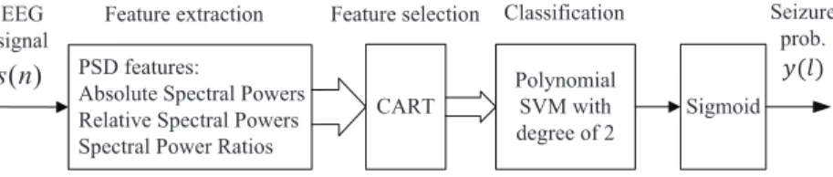
Chapter 4 develops a seizure detection algorithm for long-term fragmented EEG recordings [29]. In the proposed approach, we ﬁrst compute the spectrogram of the input fragmented EEG signals from three or four electrodes. Spectral powers and spectral ratios are extracted as features. The features are then subjected to feature selection

(34)

using classification and regression tree (CART). The selected features are then subjected to a polynomial support vector machine (SVM) classifier with degree of 2. Since all these features can be extracted by performing the fast Fourier transform (FFT) on the signals and the classifier requires low hardware complexity [97], the proposed algorithm can be implemented by the hardware with low complexity and low power consumption.

Chapter 5 develops a patient-specific algorithm that can reliably predict seizures using either one or two electrodes [27] for short-term dataset. The proposed algorithm achieves an overall sensitivity higher than 90% and a false positive (FP) rate less than 0.125 FP/hour. The algorithm also requires a low hardware complexity in extracting features and classification. In the proposed approach, we first compute the spectrogram of the input EEG signals from one or two electrodes. A window based PSD computation is used with a 4-second sliding window with half overlap. Thus, the effective window period is 2 second. Spectral powers and spectral ratios are extracted as features and are input to a classifier. A postprocessing step is used to remove undesired fluctuations of the decision output of the classifier. The feature signals are then subjected to feature selection and classification where two strategies are used. One is the single feature selec-tion and the other is the multi-dimensional feature selecselec-tion. While a seizure predicselec-tion system using a single feature requires low hardware complexity and power consumption, systems using multi-dimensional features achieve a higher prediction reliability. Multi-dimensional features are selected for patients where systems using a single feature can not achieve a predetermined requirement.

Chapter 6 develops a patient-specific algorithm that can reliably predict seizures with high area under curve (AUC) for long-term fragmented EEG recordings [81, 96]. The proposed algorithm compares the performance of different feature sets and different classifiers for different canine or human subject. In the proposed approach, we first extract two sets of features. A window based feature extraction is used, where the window size is 4 second for spectral feature set and is 10 second for the correlation feature set, respectively. The 10-second window for correlation is chosen for an accurate estimate of the correlation coefficient. The first feature set includes spectral powers and spectral ratios. The second feature set includes correlation coefficients between all possible pairs of electrodes. The two feature sets are then subjected to feature selection and classification independently. Three classifiers are used and tested on the selected

(35)

15 features, which include AdaBoost, radial basis function kernel support vector machine (RBF-SVM), and artiﬁcial neural netwroks (ANN).

1.3.2 PART II

PART II discusses feature selection methods for binary classiﬁcation and multicalss classiﬁcation.

Chapter 7 proposes a new feature selection algorithm based on minimum uncertainty and sample elimination (referred as MUSE) [98]. The three-step algorithm ﬁrst quan-tizes features into bins, ranks the features based on an uncertainty score, selects the feature with the lowest uncertainty score, and then discards samples based on an im-purity metric. The discarded samples are not used for selection of subsequent features. The process is repeated until a stopping criterion is satisﬁed.

Chapter 8 proposes a new multi-class feature selection criterion based onminimum uncertainty (referred as M3U) [99]. In this chapter, we propose a three-step algorithm that ﬁrst quantizes features into bins, computes an uncertainty vector for each feature and all sample in each feature, and ﬁnally iteratively selects features that achieves the

minimum mean minimum uncertainty (M3U). The proposed iterative feature selection algorithm includes two minimization steps and one expectation step, which include (1) ﬁnd the minimum uncertainty (MU) score for each feature sample given a feature subset, (2) compute the mean minimum uncertainty score (M2U) for the feature subset, and (3) select the feature that achieves the minimum mean minimum uncertainty score (M3U).

1.4 Contributions of the dissertation

In this section, main contribution of each part is discussed.

First, Part I introduces a novel frequency-domain model ratio (FDMR) test to identify the discriminative ratio features from a single-channel signal. Although the ratios in [30, 27] were chosen using band deﬁnitions from neuroscience, such as δ,θ,α,

β, andγ, and ranking algorithms from machine learning, the actual bands do not need to coincide with these bands. Several theoretical questions remain unanswered. Why the ratio features amplify the discrimination remains unexplained. How the two bands should be chosen to maximize the discrimination remains unknown. These questions

(36)

are answered in this Chapter 3. Using an auto-regressive model, we argue that a state change in a time-series corresponds to a change in the filter model. From the ratio of the frequency-domain characteristics of these two models, i.e., one frequency-domain response normalized with respect to the other, we can determine two bands such that for one band the ratio is much higher than 1 and for the other much less than 1. We show that the ratio of spectral powers of a single time-series in these two bands is amplified for one of the two states. This chapter shows that the effect of the non-stationarity of the noise power can be eliminated by using the ratio of spectral powers when the signal-to-noise ratio (SNR) is high. This chapter also shows that, even when the SNR is low, the ratio of spectral power ratios can significantly discriminate the state of the time-series if a postprocessing step such as a second-order Kalman filter is applied to the ratio feature. Thus, ratio of spectral powers can be used for identifying state of a non-stationary time-series assuming the model filters for the two states are different.

Second, Part I shows that combining the PSD features such as absolute spectral powers, relative spectral powers and spectral power ratios as a feature set and then carefully selecting a small number features from a few electrodes can achieve a good de-tection and prediction performances on short-term datasets and long-term fragmented datasets. Since only a few features from a few electrodes are carefully selected us-ing various feature selection method, the proposed algorithms also have a low-power and low-complexity hardware design. In low-power and low-complexity hardware de-sign, the first key consideration is the number of sensors used to collect EEG signals. Electrode selection is an essential step before feature selection as sensors and analog-to-digital converters (A/D) can be highly power consuming for an implantable or wearable biomedical device. The second key consideration is selecting useful features that are computationally simple and are indicative of upcoming seizure activities. The third key consideration is the choice of classifier. Based on the selection of the classifier, a criteria for electrode and feature selection should be chosen accordingly in order to achieve the best classification performance.

Part II proposes novel feature selection methods for binary classiﬁcation (MUSE) and multi-class classiﬁcation (M3U). The main contribution of MUSE is that a new feature selection algorithm based on minimum uncertainty and sample elimination (re-ferred as MUSE) is proposed. The sample elimination process reduces redundancy and

(37)

17 the selection of a feature with the least uncertainty score increases relevance. The dis-carding of the samples and the selection of the feature are both nonlinear operations and are ideal for general machine learning applications where feature samples may not necessarily be linearly separable. The main contribution of M3U is a new multi-class feature selection criterion based onminimum uncertainty. To the best of our knowledge, the one-versus-all (OVA) uncertainty vector is deﬁned in M3U is is a new sample-wise criterion that has not been proposed before. Given a feature sample in a particular feature, this uncertainty score illustrates how good the bin (corresponding to the fea-ture sample) is to separate the class (corresponding to the feafea-ture sample) from the remaining classes.

(38)

Part I

Feature Identiﬁcation, Extraction

and Classiﬁcation

(39)

Chapter 2

Seizure Detection from

Short-Term EEG Recordings

using Wavelet Decomposition of

the Prediction Error Signal

Our main objective is to develop an automated algorithm that can reliably detect seizures. The algorithm should also have a low hardware complexity. In the proposed approach [31], only a single channel EEG signal is analyzed for seizure detection. We first filter the EEG signal by a prediction error filter, also known as a whitening filter, to compute an error signal. A 19th-order prediction error filter (PEF) computes the error signal as the difference between the current input sample and the estimate of it. A window based processing is used with a 2-second sliding window with half overlap. The predictor coefficients are recomputed every one second. A two-level wavelet decompo-sition of the error signal computes the approximate signal and two detail signals. The total energies in a window of the error signal and the three signals from the wavelet de-composition are extracted in two different ways. The features are input to two types of classifiers: a linear support vector machine (SVM) classifier and an AdaBoost classifier. The performance of each classifier is evaluated and compared against the other.

(40)

2.1 Materials and Methods

2.1.1 Patients Database

We have trained and tested our algorithm on the Freiburg EEG database [100], which is available to any lab by request. According to [100], this database contains electrocor-ticogram (ECoG) or iEEG from 21 patients with medically intractable focal epilepsy. We have chosen 18 of the available datasets of 21 patients, who have three or more seizures (the minimum number for cross-validation). Each 2-s-long window of iEEG has been categorized as ictal (containing a seizure), interictal (at least 1 h preceding or postceding a seizure), preictal (in 60 min preceding a seizure onset), or artifact. Half an hour of iEEG recordings preceding preictal and an hour of those postceding seizure offset are excluded in training. The Freiburg database contains six of iEEG recordings from grid, strip, or depth-electrodes, three near the seizure focus (focal) and the oth-er three distal to the focus (afocal). Seizure onset times and artifacts woth-ere identified by certified epileptologists. The data were collected at 256 Hz (Patient 12 at 512 Hz) sampling rate with 16 bit analog-to-digital converters.

2.1.2 System Architecture Classifier Prediction Error Filter w(n) Wavelet Decomposition EEG signal s(n) Error Signal e(n) +1 0 Feture Vectors ݂ሺ݈ሻ Feature Extractor e(n),or Wavelet Coefficients a(n) or di(n) Esitimate Prediction Error Filter Coeffcients w(n) ݈ ݕሺ݈ሻ

Figure 2.1: System architecture for seizure detection

Fig. 2.1 shows the overall system for seizure detection. Lets(n) denote the single-channel iEEG signal. First the signals(n) is windowed and ﬁltered by a prediction error ﬁlter to compute the error signal e(n). A two-level wavelet decomposition is applied to the error signal to obtain one approximate signal and two detail signals. An 8-dimensional feature vector f(l) = [f1(l), f2(l), ..., f8(l)]T is extracted by computing the

(41)

21 total power for the error signal and the three signals obtained by wavelet decomposition inside the sliding window. The feature vectors are then subjected to training and classiﬁcation. The output of the systemy(l) represents the detection signal. Two types of classiﬁers are considered. These include: the linear SVM and the AdaBoost. The training follows leave-one-out procedure, where the seizure to be tested is not used for training.

2.1.3 Feature Extraction

This section describes the method for feature extraction, which includes prediction error ﬁlter, a 2-level wavelet decomposition and power computation.

Window-based signal processing

The input signal is divided into the input segments (or windows) and the signal is processed segment by segment. Each segment has a 50% overlap with its neighbour segment.

Preprocessing

In the first step, EEG data is preprocessed to remove its mean. The demeaned signal is then filtered by a PEF to remove the predictable component of the EEG signal. Each window is 2 seconds long and has 50% overlap. The PEF is then used to compute the error signal for next one second. Thus, effective feature computation rate is one per second.

Let wf represent tap-weights vector of an m-tap predictor (or a mth-order PEF).

Coeﬃcients of the PEF can be computed by solving the Wiener-Hopf equation: wf = R−1r, where R represents the autocorrelation matrix of the input sample vector of a window, and r represents the cross-correlation vector between the input sample vector and its delayed versions. Levinson-Durbin algorithm is used to solve the above equation [101].

A 19th-order PEF is chosen for this dataset. A singular value decomposition of the covariance matrix is performed for patient No. 1 to ﬁnd the optimal order of the predictor. Fig. 2.2(a) and Fig. 2.2(b) show the plots of the percentage of total energy

(42)

captured by the predictor versus the predictor’s order using (a) an hour’s inter-ictal data from patient No. 1 while the patient is awake and (b) an hour’s inter-ictal data from patient No. 1 while the patient is sleeping, respectively. A 19-tap predictor (equivalently, 19th order or 20-tap PEF) can capture about 95% of the total energy of the signal. 0 10 20 30 40 20 30 40 50 60 70 80 90 100 No. of SV Total energy (%) awake 0 10 20 30 40 20 30 40 50 60 70 80 90 100 No. of SV Total energy (%) sleep

Figure 2.2: Percentage of total energy captured by the predictor versus the predictor’s order using (a) an hour’s inter-ictal data from patient No. 1 while the patient is awake and (b) an hour’s inter-ictal data from patient No. 1 while the patient is sleeping.

Figure 2.3: Spectrograms of the EEG signal (left) and its error signal (right) using interictal recordings for the 16th hour from patient No. 1.

Fig. 2.3 shows the spectrograms of the EEG signal and its error signal corresponding to the interictal recordings for patient No. 1 in the 16th hour, where undesired harmonics in the interictal period are ﬁltered and the dominance of the low frequencies on the total power is eliminated after prediction error ﬁltering.

(43)

23

Discrete wavelet decomposition

A two-level wavelet decomposition is applied to the error signal to compute wavelet coeﬃcients at diﬀerent levels.

Feature extractor

Two types of features are extracted from the error signal and the wavelet coeﬃcients: one is the total power and the other is the sum of the logarithm of the absolute feature values (also equivalently, logarithm of the product of the absolute feature values). Total power for each segment is obtained by computing the sum of the squared value of the wavelet coeﬃcients (or the error signal). Mathematically, these are computed as:

f′(l) =∑ n∈Il log|e(n)| (2.1) f′′(l) =∑ n∈Il e2(n) (2.2)

where Il = {(l−1)fs+ 1, ..., lfs} represents the samples of the l-th window. Fig. 2.4

shows the block diagram of feature extraction, where a total number of 8 features (f1(l)

to f8(l)) are extracted from the error signal, e(n), and the wavelet coeﬃcients, a2(n),

d2(n), and d1(n); four of these features represent the mean power and the remaining

four represent the logarithm of the product of the absolute values. For the AdaBoost classifier, all 8 features are input to the classifier. The classifier always selects between 1 to 4 out of the 8 features.

d1(n) a2(n) d2(n) e(n) Accumu-lator ݈݋݃ȁ ή ȁ ሺήሻʹ _ሺήሻʹ _ሺήሻʹ _ሺήሻʹ Accumu-lator Accumu-lator Accumu-lator ݈݋݃ȁ ή ȁ ݈݋݃ȁ ή ȁ ݈݋݃ȁ ή ȁ Accumu-lator Accumu-lator Accumu-lator Accumu-lator f1(l) f2(l) f3(l) f4(l) f5(l) f6(l) f7(l) f8(l)

(44)

2.1.4 Seizure Detection Classiﬁcation

Two classification methods are used and their performances are compared. One is classification using a linear Support Vector Machine (SVM) and the other by using AdaBoost. These classifiers can be easily implemented in hardware with low power consumption.

2.2 Experimental Results

Table 2.1: Detection Performance of The System using linear SVM

Patient electrode Total No. Sensi- No. of FP

No. No. of SZ tivity FP rate

1 1 4 100 1 0.042 3 1 5 100 4 0.167 4 1 5 100 0 0 5 1 5 100 14 0.583 6 2 3 100 13 0.542 7 1 3 100 0 0 9 1 5 100 3 0.125 10 2 5 100 0 0 11 1 4 100 1 0.042 12 1 4 100 0 0 14 1 4 100 0 0 15 1 4 75 0 0 16 3 5 80 8 0.333 17 1 5 100 0 0 18 1 5 100 5 0.208 19 1 4 50 2 0.083 20 1 5 100 1 0.042 21 1 5 100 0 0 Overall 80 95 53 0.124

The parameters for the system are described as follows:

1) For each patient, we apply our algorithms on all electrodes. We select the electrode with best performance.

2) Leave-one-out cross validation is used where one seizure is left out for testing and the classiﬁer is trained using features corresponding to the remaining seizures that constitute the training set. This is repeated with each seizure left out once for testing. The classiﬁer with the best performance over the entire data is selected.