Tree Species Classification by Fusing of very high-resolution Hyperspectral Images and 3K-DSM

TREE SPECIES CLASSIFICATION BY FUSING OF VERY

HIGHRESOLTUION HYPERSPECTRAL IMAGES AND 3K-DSM

Remote Sensing Technology Institute (IMF), German Aerospace Center (DLR), 82234 Weßling, Germany

ABSTRACT

Tree species information is crucial in sectors such as forest management and nature conservation. It is often required over a large area. In this study, tree species classification was performed using hyperspectral data and the Digital Surface Model generated from DLR-3K aerial borne stereo camera System. In the classification step, pixel-based approach and the patch-pixel-based approach with Bag-of-Word (BoW) model were proposed and tested. The two approaches have been performed in the Kranzberg Forest near Munich, Germany. The comparison was taken in a statistical way. By using proper features combination, the pixel-based classification can achieve very high accuracy (Kappa =0.95), while the patch-based method only has accuracy around 60%.

Index Terms— Hyperspectral, Tree Species, Random Forests, BoW, DSM

1. INTRODUCTION

Sustainable forestry management has been widely recognized as the principle objective of forest policy and practice in Europe. Tree species classification with remote sensing data is motivated by the need of various research and work in the forest management and conservation sectors [1]. Those needs include forest inventory, biodiversity assessment and monitoring [2], hazard and stress estimation [3]. Moreover, accurate forest species map is also prerequisite to fire propagation simulation models and fire risk assessment [4]. Knowledge on tree species distribution in turn could also affect forest harvesting and management policies [4][5].

Therefore, remote-sensing assisted tree species classification is desired by many sectors and has been extensively studied in recent years. The advancement of remote sensing technology has enabled rapid growing in research on tree species classification in the last 35 years [6]. Comparing to the traditional field survey, remote sensing is more suitable for inaccessible and very large areas; it also consumes much less time and manpower. Hyperspectral data have been used to map tree species in some researches due to their higher spectral range and resolution. According to a literature review about research on tree species classification from year 1980 to 2014 [7],

most cases were hyperspectral or imaging spectroscopy studies; the second most used is multispectral. Many studies have adopted multi-sensor data. For instance, active system such as Light Detection and Ranging (LiDAR) together with passive ones. During the last ten years, the exponential growth of tree species classification corresponds to the increased availability of hyperspectral data and LiDAR data [7]. Both data have been frequently utilized in forest inventory context, where tree species classification is the most popular target variable, in addition to total growing stock volume and biomass [7].

In earlier studies, most widely used classification techniques include supervised maximum likelihood classifier (MLC), and unsupervised clustering such as K-means and ISODATA [7][8][9]. Since 1995, with the methodological developments in the domain of statistical learning, classification algorithms have evolved to non-parametric decision tree based classifiers and neural networks. Recent studies using mixed or transformed input features (spectral, texture, geometric, vegetation indices) have employed non-parametric machine learning methods such as Random Forests (RF) and Support Vector Machine (SVM) [7][10][11]. Recently, the patch-based Bag-of-word texture-classification has achieved good performance in object detection [12] and has been tested for aerial image based crowd [13] and landcover classification [7]. According to the authors’ knowledge, it has not yet been tested for hyperspectral image based tree species classification.

The specific objectives of this paper include evaluating of various feature combination for the RF classification validate if height information improves accuracy, and introducing patch-based Bag-of-Word method for tree species classification and comparing the results from RF.

2. RESEARCH SITE AND DATASETS 2.1. Research site

The study site is located approximately 35 km northeast of Munich in Kranzberg Forest. The forest comprises mainly of European beech (Fagus sylvatica) and Norway spruce (Picea abies). Outside of the forest boundary there are some houses, field and asphalt highway. Within the forest there are some gravel roads for human access. The Kranzberg forest is a university research site since 1992. The site is

equipped with scaffoldings and a canopy crane system, which allows for easier data acquisition and observation.

The main purpose of our research is to accurately extract the tree species in the forest to provide valuable information to the research team on the study site who is studying the reaction of tree species to exacerbating summer drought. The region of interest has a size of 840 × 840 m2_, and is in the center of Kranzberg forest. And tree species classes we are interested in are spruce (Picea abies) and beech (Fagus sylvatica).

2.2. Hyperspectral data

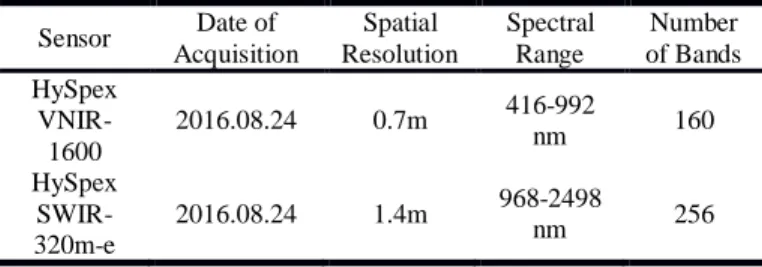
The hyperspectral images used in this paper were acquired by imaging spectrometer system HySpex on 24th of August 2016. HySpex system is purchased from the Norwegian company Norsk Elektro Optikk A/S (NEO) [14]. With two individual sensors, the system covers visible near-infrared (VNIR) and short wave infrared (SWIR) spectral domains ranging from 0.4 to 2.5 nm. Hyperspectral images are orthorectified with SRTM because of the alignment problem in 3K 3D model. The spatial resolution of HySpex data is summarized in table1. The system is equipped with a high precision iTraceRT-F200 coupled INS/GPS navigation system that provides accurate georeferencing for the acquired data. A calibration flight is carried after installation onto an aircraft over an area with known reference points [14].

Table 1. Theparameter of the two sensors of the HySpex system

Sensor Date of Acquisition Spatial Resolution Spectral Range Number of Bands HySpex VNIR-1600 2016.08.24 0.7m 416-992 nm 160 HySpex SWIR-320m-e 2016.08.24 1.4m 968-2498 nm 256 2.3. 3K Data

In this study, we use a very high resolution aerial dataset to generate digital surface model (DSM). The aerial imagery dataset was acquired by the DLR 3K sensor system at the same flight with HySpex system. The 3K system consists of three cameras (nadir, forward and backward), which enables capturing of multi-view along-track images with the resolution of 13 centimeters [14].

3. METHODOLOGY

In this paper, pixel-based and patch-based method are tested and briefly introduced below.

3.1. Pixel-Based Method 3.1.1 Random Forests (RF)

RF is an ensemble learning method that fits many of decision tree classifiers on various sub-samples of the input dataset and vote to decide the class (In the case of

regression, averaging is used). Error rate can be estimate using out-of-bag (OOB) method that is based on the training data. RF classifier has been widely used in tree species classification context, including landcover classification and forest type mapping [7].

3.1.2 Features

Features used in the experiment are the original hyperspectral images, Maximum Noise Fraction (MNF) components, three vegetation indexes and DSM.

MNF

The abundance of spectral information also brings redundancy. In hyperspectral images, neighboring bands are often highly correlated, which not only add unnecessary information but also add to the computational complexity when processing. Also, many bands in hyperspectral images can be noisy. Therefore, dimensionality reduction of hyperspectral images is a desired state-of-art method. Maximum Noise Fraction (MNF) transformation [15] is a linear transformation consisting of two PCA rotations and a noise whitening step. The returned data contains the most informative bands.

Landcover Features

Thanks to the high spectral resolution, we can have reflectance/radiance values with very fine resolution. Therefore, many vegetation indexes could be calculated accurately. For the experiment, we have selected three vegetation indexes (VI) as landcover features.

Normalized Difference Vegetation Index (NDVI). NDVI is calculated as follows:

NDVI = (NIR — VIS) / (NIR + VIS)

In our dataset, NIR is the reflectance at wavelength 858 nm; VIS is the reflectance at wavelength 649 nm [16].

Red Edge NDVI (redNDVI)

The redNDVI is an adapted version of NDVI. Red edge is the region in spectrum between 680 and 750 nm where the reflectance change of vegetation is the sharpest[17].

𝑟𝑒𝑑𝑁𝐷𝑉𝐼 =(𝜆750µm− 𝜆705µm) (𝜆750µm+ 𝜆705µm

Red Edge Reflection Point (REIP)

This parameter correlates well with total chlorophyll content at leaf level [18]. It is calculated as follow:

𝑅𝐸𝐼𝑃 = 700 + 40(

(𝜆670µm+ 𝜆780µm)

2 − 𝜆700µm

𝜆740µm− 𝜆700µm ) Reflectance measurements at 670nm and 780nm are used to estimate the inflection point reflectance[19].

By incorporation VI with other features, the non-vegetation components can be easily separated from trees of interest.

Height Features

In this paper, DSM with the resolution of 20 cm is generated from the 3K data. It is resampled to the same resolution as the hyperspectral data. This height information is then served as an additional feature in the pixel-based classification. To find out the best feature combinations, we

have tested six different combinations as the features to the RF classifier:

1) Original hyperspectral image (160 bands) 2) MNF transformed image with 50 bands 3) MNF and VI (NDVI, redNDVI and REIP) 4) MNF and DSM

5) VI and DSM 6) MNF, DSM and VI 3.2. Patch-Based Method

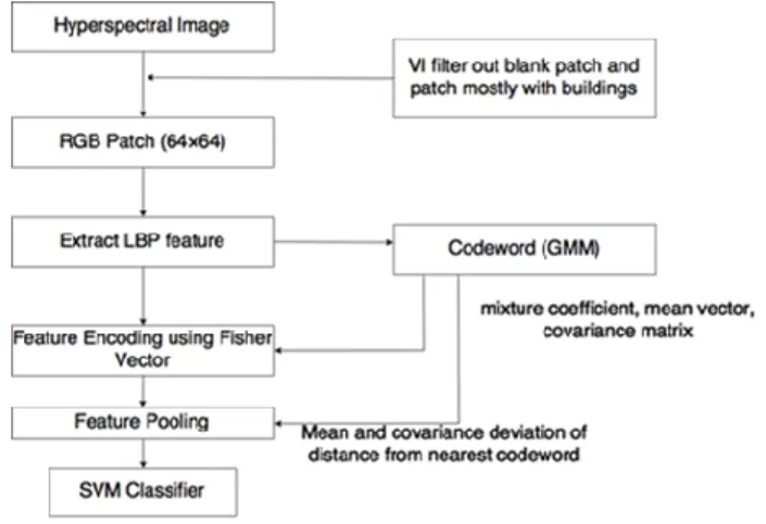
Different from pixel-based, patch based method focus more on utilizing the texture information within an area. Here a Bag-of-Visual-Word (BoW) method is used. BoW as a framework of four general processing steps, which follow on the patch sampling. It comprises mainly of four steps: local feature extraction, codeword generation, feature encoding and feature pooling [13].

Features are extracted using Local Binary Pattern (LBP). LBP labels pixels by comparing them with central pixel of a 3×3 window and assign 1 to pixels having gray value greater than central pixel and 0 to pixels that are smaller. For each surrounding pixel, a weight of 2 to the power of its rank was given according to its relative position to the central pixel. In total, there are 256 different values for a pixel and window size of 3×3. The number of occurrences of each label represented in a 256-bin histogram can be used as a texture descriptor. To reduce computational complexity, an extension of LBP called uniform pattern was used, where the shifts between 1 and 0 happen at most twice. The resulting feature matrix 𝑋𝑝 of local feature vector Xn∈Rm _{has a reduced dimension of m=58. This improved} descriptor has better classification capacity while reducing the computational complexity.

After extracting all local features, a randomly sampled subset X of these local features is used for generating the codeword using Gaussian Mixture Model (GMM), which is created by expectation maximization and a pre-defined number of cluster centers. GMM can be treated as the representative model of the whole feature space where cluster centers represent codeword in a dictionary [13].

After the generation of GMM, each patch feature 𝑋𝑝 =

[𝑥, … , 𝑥𝑛] is encoded using Improved Fisher Vector (IFV) [20]. Descriptor can be modeled by GMM by being weighed with mode k in the mixture with a posterior probability qnk that is defined as:

𝑞𝑛𝑘=

exp [−1₂(𝑥𝑛−𝑑𝑘)𝑇∑ (𝑥−1𝑘 𝑛−𝑑𝑘)]

∑𝑡=1𝐾 exp [−1₂(𝑥𝑛−𝑑𝑡)𝑇∑ (𝑥−1𝑡 𝑛−𝑑𝑡)] (1)

qnk can be regarded as the influence of a mode k on the final feature encoding of local feature xn. It is an element of the assignment matrix 𝑄𝑝 = [𝑞1, … , 𝑞𝑛] that assigns a weight of every mode k to each feature descriptor xn [13].

We used the size of 64×64 pixels for the patch preparation. Besides the image used in pixel-based method, more patches are generated from the image stripe from the

same flight to generate enough patch for training and testing.

Figure 1. Work flow of patch-based method. 4. EXPERIMENTAND RESULT 4.1. Experiment

The accuracy of pixel-based method is evaluated with ground truth data to get species-specific accuracy score even though RF classifier can estimate error by OOB with only training data. Training sample and test sample consist of 8.6% and 61.7% of total number of pixels respectively. The performance of classifier is evaluated by overall accuracy, Cohen’s Kappa score, build-in OOB and accuracy for each species. There are in total 6 classes in the image: spruce, beech, grass, road, shadow and soil.

For patch based method, each patch is manually assigned to one of four classes to create the ground truth. Classification is performed by SVM. SVM is trained with 20 and 200 training respectively.

Class1 Spruce if patch is monoculture or other species is less than 10% of coniferous tree besides shadow

Class2 Beech if patch is monoculture or other species is less than 10% of this broad leaf and deciduous tree besides shadow

Class3 Mixed If one tree species is more than 10% of another tree species when shadow is excluded.

Class4 Others patch is defined as this class if more than 80% of the patch contains non-tree object (except shadow).

4.2. Results

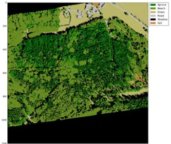
The results for two methods are summarized in Table 2 and Table 3. For patch based method, the highest overall accuracy was achieved by using MNFDSMVI feature. It also achieved the highest accuracy for Cohen’s Kappa, OOB, spruce, grass and road. The best result for beech was achieved by using only MNF feature. In general, height information can help to improve the accuracy, but the contribution was not significant in our experiment, even not as much as that of VI. VI is also good at differentiating between non-vegetation and vegetation objects. Figure 2

Table 2: Result of the pixel-based tree species classification

Overall Kappa OOB Spruce Beech Grass Road Shadow Soil

All bands 93.73% 91.44% 98.07% 78.84% 93.83% 99.84% 95.54% 99.47% 83.60% MNF 96.15% 94.73% 98.41% 84.44% 98.10% 99.39% 96.40% 97.73% 96.16% MNF VI 96.21% 94.82% 98.66% 85.04% 97.59% 99.68% 97.55% 98.12% 96.30% MNFDSM 96.33% 94.98% 98.66% 84.69% 97.77% 99.91% 96.40% 98.68% 96.30% DSM VI 88.40% 84.24% 97.33% 69.85% 85.80% 99.82% 98.68% 93.41% 92.11% MNFDSMVI _{96.38% 95.05% 98.77% 85.50% 97.36% 99.91% 97.58% 98.91% 96.65%}

Table 3: The classification accuracy of patch-based BoW method

20 Training samples (4 Classes) 200 Training samples (4 Classes)

Round 1 2 3 Average 1 2 3 Average

Overall Accuracy 66.23% 62.25% 61.38% 63.28% 80.84% 78.91% 76.95% 78.90% Mixed 14.57% 22.61% 84.92% 40.70% 63.64% 66.88% 62.99% 64.50% Beech 6.96% 2.53% 20.25% 9.92% 57.52% 66.37% 59.29% 61.06% Other 83.01% 79.62% 83.79% 82.14% 93.22% 92.96% 93.92% 93.37% Spruce 56.33% 49.65% 28.95% 44.98% 66.23% 60.11% 54.40% 60.25% SD 2.58 1.95

shows the best result of RF by using the MNF, DSM and VI as input features. The result is satisfactory. It clearly simulated the silhouette of trees and other components. For the patch-based classification. In group of 20 training samples, the accuracy fluctuates drastically. This is due to the insufficiency of training data. The results stabilized when increasing number of training sample to 200. The best accuracy was achieved in ‘Other' class. This fact is attributed to the distinct local features in those image patches. For other classes, the accuracy is around 60%.

Figure 2. Classification result of pixel-based method using MNFDSMVI as the feature

Table 2 briefly summarized some misclassification examples of patch based method and compared them with pixel-based result cropped to the same size. The experiment area can be divided into 324 patches (251 non-blank). In total 192 patches are correctly classified. As these examples

show, it is sometimes very difficult to properly label a patch in the forest. For example, the first example was labeled as mixed, but was half covered by Beech. Therefore, it was wrongly classified as Beech by the patch-based method.

Table 4. Some misclassification examples

True Label Mixed Beech Other Spruce

Original patch Pixel-based result Pixel percentage 17.7% spuce 49.1% beech 33.2% shadow 6.3%spruce 77.0%beech 15.5% shadow 95.4%grass 4.4% road 46.8% spuce 2.88%beech 50.0% shadow Patch-based

prediction Beech Mixed Spruce Beech

5. CONCLUSION

In this work, we have fused the hyperspectral data and the DSM from aerial stereo data for tree species classification. Both pixel-based RF classification and the patch-based texture classification methods have been tested. The pixel-based method outperformed the patch-pixel-based method by a very high percentage. Also, pixel-based method provides tree species information to the pixel level, which allows more flexibility in the application of classification results. The better result achieved by pixel-based method suggest that hyperspectral imagery has high potential in tree species classification where the spectral difference across species is subtle. The less accurate classification result from patch-based method suggests that texture information alone is not sufficient for tasks such as tree species classification. However, it is quite time consuming to prepare proper training data for the pixel-based classification method. A combination of the pixel- and patch-based classification approaches will be further exploited in our future study.

6. REFERENCES

[1] European Environmental Agency, 2007. “European Forest Types: Categories and Types for Sustainable Forest Management Reporting and Policy,” EEA

Technical Report No 9/2006, EEA, Copenhagen, 2006.09. [2] X. Shang, L. A. Chisholm, “Classification of Australian

Native Forest Species Using Hyperspectral Remote Sensing and Machine-Learning Classification

Algorithms,” IEEE Journal of Selected Topics in Applied Earth Observations and Remote Sensing 2014, 7 (6), pp. 2481–2489, 2014.

[3] Wu, C., Niu, Z., Tang, Q., Huang W., “Estimating Chlorophyll Content from Hyperspectral Vegetation Indices: Modeling and Validation,” Agricultural and Forest Meteorology 2008, 148 (8), pp. 1230–1241. 2008. [4] Keramitsoglou, I., Kontoes, C., Sykioti, O., Sifakis, N.,

Xofis, P. “Reliable, Accurate and Timely Forest Mapping for Wildfire Management Using ASTER and Hyperion Satellite Imagery.” Forest Ecology and Management 2008, 255 (10), pp. 3556–3562.

[5] Dalponte, M., Bruzzone, L., Gianelle, D., “2012. Tree species classification in the Southern Alps based on the fusion of very high geometrical resolution

multispectral/hyperspectral images and LiDAR data”. Remote Sens. Environ. 123 (0), pp. 258–270.

[6] Plourde, L.C., Ollinger, S.V., Smith, M.-L., Martin, M.E., 2007. Estimating species abundance in a northern temperate forest using spectral mixture analysis. Photogramm. Eng. Remote. Sens. 73 (7), 829–840. [7] Fassnacht, F. E., Latifi, H., Stereńczak, K., Modzelewska,

A., Lefsky, M., Waser, L. T., Straub, C., Ghosh, A. “Review of Studies on Tree Species Classification from Remotely Sensed Data,” Remote Sensing of

Environment 2016, 186, pp. 64–87.

[8] Moore MM, Bauer ME. “Classification of forest vegetation in north-central Minnesota using Landsat Multispectral Scanner and Thematic Mapper data,” Forest Science. 36(2), pp. 330-42, 1990 Jun 1. [9] Walsh, S.J., “Coniferous tree species mapping using

LANDSAT data,” Remote Sens. Environ. 9 (1), pp. 11– 26, 1980

[10]Immitzer, M., Atzberger, T.C., Koukal, 2012b. “Suitability of WorldView-2 data for tree species classification with special emphasis on the four new spectral bands,” Photogrammetrie, Fernerkundung, Geoinformation, pp. 573–588, 2012.05.

[11]Pant, P., Heikkinen, V., Hovi, I.A., Korpela, Hauta-Kasari M., Tokola, T., „Evaluation of simulated bands in airborne optical sensors for tree species identification,” Remote Sens. Environ. 138 (0), pp. 27–37. 2013 [12]Lazebnik, S., Schmid, C. and Ponce, J., “A sparse texture

representation using local affine regions,” IEEE Transactions on Pattern Analysis and Machine Intelligence, 27(8), pp.1265-1278, 2005.

[13]Meynberg, O., Cui, S., Reinartz, P, “Detection of High-Density Crowds in Aerial Images Using Texture Classification,” Remote Sensing 2016, 8 (6), pp. 470.

[14]Köhler CH. “Airborne Imaging Spectrometer HySpex,” Journal of large-scale research facilities JLSRF. pp. 1-6, 2016 Nov 18.

[15]Green, A.A., Berman, M., Switzer, P. and Craig, M.D., “A transformation for ordering multispectral data in terms of image quality with implications for noise removal,” IEEE Transactions on geoscience and remote sensing, 26(1), pp.65-74, 1988.

[16]Rouse, J. W., Jr., Haas, R. H., Schell, J. A., Deering, D. W. “Monitoring vegetation systems in the Great Plains with ERTS. NASA”. Goddard Space Flight Center 3d ERTS-1 Symposium., Vol. 1, Sect. A, pp. 309-317. [17]Gitelson, A., Merzlyak, M. N. “Spectral Reflectance

Changes Associated with Autumn Senescence of Aesculus Hippocastanum L. and Acer Platanoides L. Leaves Spectral Features and Relation to Chlorophyll Estimation,” Journal of Plant Physiology 1994, 143 (3), pp. 286–292.

[18]Vogelmann, J.E., Rock, B.N. and Moss, D.M., “Red edge spectral measurements from sugar maple leaves,” REMOTE SENSING, 14(8), pp.1563-1575, 1993. [19]Guyot, G., Baret, F., and Major, D. J., “High spectral

resolution: Determination of spectral shifts between the red and infrared,” International Archives of

Photogrammetry and Remote Sensing, 1998.

[20]Perronnin, F., Sánchez, J., Mensink, T. “Improving the Fisher kernel for large-scale image classification,” In Computer Vision ECCV 2010, Daniilidis, K., Maragos, P., Paragios, N., Eds., Springer: Berlin, Germany, 2010, Volume 6314, pp. 143–156.