Cluster-Based Boosting

(1)

DigitalCommons@University of Nebraska - Lincoln

CSE Journal Articles

Computer Science and Engineering, Department of

2015

Cluster-Based Boosting

L. Dee Miller

University of Nebraska-Lincoln

Leen-Kiat Soh

University of Nebraska-Lincoln, [email protected]

Follow this and additional works at:

https://digitalcommons.unl.edu/csearticles

This Article is brought to you for free and open access by the Computer Science and Engineering, Department of at DigitalCommons@University of Nebraska - Lincoln. It has been accepted for inclusion in CSE Journal Articles by an authorized administrator of DigitalCommons@University of Nebraska - Lincoln.

Miller, L. Dee and Soh, Leen-Kiat, "Cluster-Based Boosting" (2015).CSE Journal Articles. 120. https://digitalcommons.unl.edu/csearticles/120

(2)

Cluster-Based Boosting

L. Dee Miller and Leen-Kiat Soh,

Member, IEEE

Abstract—Boosting is an iterative process that improves the predictive accuracy for supervised (machine) learning algorithms. Boosting operates by learning multiple functions with subsequent functions focusing on incorrect instances where the previous functions predicted the wrong label. Despite considerable success, boosting still has difficulty on data sets with certain types of problematic training data (e.g., label noise) and when complex functions overfit the training data. We propose a novel cluster-based boosting (CBB) approach to address limitations in boosting for supervised learning systems. Our CBB approach partitions the training data into clusters containing highly similar member data and integrates these clusters directly into the boosting process. CBB boosts

selectively(using a high learning rate, low learning rate, or not boosting) on each cluster based on both the additional structure provided by the cluster and previous function accuracy on the member data. Selective boosting allows CBB to improve predictive accuracy on problematic training data. In addition, boosting separately on clusters reduces function complexity to mitigate overfitting. We provide comprehensive experimental results on 20 UCI benchmark data sets with three different kinds of supervised learning systems. These results demonstrate the effectiveness of our CBB approach compared to a popular boosting algorithm, an algorithm that uses clusters to improve boosting, and two algorithms that use selective boosting without clustering.

Index Terms—Artificial intelligence, machine learning, clustering algorithms

Ç

1 I

NTRODUCTION

B

OOSTING is an iterative process used to improve the predictive accuracy for functions that supervised learn-ing (SL) systems learn uslearn-ing trainlearn-ing data. More specifi-cally, the boosting process learns multiple functions from the same SL system. Boosting then predicts the label for new data instances using a weighted vote over all the func-tions. By combining multiple functions together, boosting achieves a more refined decision boundary on the training data than using a single function.

There exists a large body of previous work that demon-strates the effectiveness of boosting. Theoretical results have shown that boosting is resistant to overfitting—a com-mon SL problem where the algorithm overspecializes on nuances in the training data to the degree that predictive accuracy on new data instances is reduced [1], [2], [3]. Fur-thermore, empirical results on a wide variety of existing data sets have shown that boosting generally achieves higher predictive accuracy than using a single function from the same SL system [4]. In addition to benchmark data sets, boosting has also been used effectively on a wide range of applications [5], [6] including engineering applications [7]. Examples of boosting applied to engineering applica-tions include using boosted funcapplica-tions to predicting concrete strength [8] and in monitoring wind turbines [9].

Despite considerable success, conventional boosting such as AdaBoost (hereafter boosting) is still not perfect. Boosting has difficulty with certain types of problematic training data including (1) training data with label noise—where the

labels of the instances provided are actually wrong—and (2) training data with what we term troublesome areas— where the relevant features of the instances are different from the rest of the training data.

First, suppose the initial function failed to predict the label correctly for certain instances, not because the initial function learned was incorrect, but because these instances were labeled wrong to begin with. However, boosting does not realize that the labels were wrong and, thus, holds the initial function responsible. As a result, boosting focuses subsequent functions on learning how to “correctly” predict these instances assuming that the wrong labels provided are correct [10], [11]. Thus, this eventually leads to boosting learning functions fitting the noise.

On the other hand, suppose that the labels provided are not noisy, but there areareas of instances where their relevant features are different from the rest of the training data. For exam-ple, suppose in an area, say, A1, features F1 and F2 are the relevant features used to determine the labels for the instan-ces, whereas, in the rest of the training data features F2, F3, and F4 are the relevant features. The initial function learned on all the training data uses F2, F3, and F4 to predict the labels for all data instances including area A1. By using features irrelevant to area A1 (i.e., F3 and F4), the initial function could struggle to predict correctly the labels for instances in A1. To complicate matters, different instances in area A1 might appear similar—because of the irrelevant features F3 and F4—but still have different labels. We refer to areas such as A1 astroublesome areasin this paper. Because of these troublesome areas, boosting cannot rely on the initial function to make a good decision about what instances are correctly labeled and incorrectly labeled. This is a problem because boosting focuses on instances that were incorrectly labeled by the initial function. Using only the incorrectly labeled instances, boosting has difficulty learning accurate subsequent functions for troublesome areas. Note that in real-world data sets, a number of factors

The authors are with the Computer Science and Engineering Department, University of Nebraska, Lincoln, NE 68588.

E-mail: {lmille, lksoh}@cse.unl.edu.

Manuscript received 21 May 2014; revised 11 Nov. 2014; accepted 8 Dec. 2014. Date of publication 17 Dec. 2014; date of current version 27 Apr. 2015. Recommended for acceptance by S. Yan.

For information on obtaining reprints of this article, please send e-mail to: reprints.org, and reference the Digital Object Identifier below.

Digital Object Identifier no. 10.1109/TKDE.2014.2382598

IEEE TRANSACTIONS ON KNOWLEDGE AND DATA ENGINEERING, VOL. 27, NO. 6, JUNE 2015 1491

1041-4347ß2014 IEEE. Personal use is permitted, but republication/redistribution requires IEEE permission. See http://www.ieee.org/publications_standards/publications/rights/index.html for more information.

DOI: 10.1109/TKDE.2014.2382598

(3)

could result in troublesome areas, including the presence of (1) lower dimensional manifolds of relevant features [12], (2) multiple views (i.e., groups) of relevant features [13], and (3) instances collected from multiple tasks (i.e., distribu-tions) with different sets of relevant features [14].

Furthermore, boosting can still have difficulty when the SL system learns complex functions overfitting the training data [15], [16]. Boosting uses all these functions together when predicting the label for new instances. As a result, overfitting in functions is effectively propagated into boosting.

One explanation for why boosting has problems is the way it learns subsequent functions. These functions are trained focusing on all the incorrect instances in the train-ing data where the initial function did not predict the cor-rect label. This additional training forces subsequent functions to accommodate highly dissimilar training data. This can result in subsequent functions with an increased complexity and likelihood of overfitting. At the same time, the training process for these subsequent functions tends to ignore problematic training data on which the initial function predicted the correct label. This can result in important information withheld from subsequent func-tions such as the labels for correct instances that are highly similar to the incorrect instances.

To address the limitations of boosting, we hereby pro-pose a novel cluster-based boosting (CBB) approach that incorporates clusters into the boosting process to improve how boosting learns these subsequent functions. Our CBB approach partitions the training data into clusters that con-tain highly similar member data to break up and localize the problematic training data. CBB then uses these clusters integrated into boosting to improve the subsequent func-tions as opposed to previous work that has used clusters only for preprocessing [17]. First, CBB evaluates each cluster separately to identify whether the problematic training data should be used to learn subsequent functions. This allows for more selective boosting to accommodate different types of problematic training data. Next, CBB learns subsequent functions separately on each cluster using only the member data in that cluster. This allows for less complex subsequent functions and helps to mitigate overfitting from being prop-agated into boosting. Last, CBB learns subsequent functions starting with all the cluster members—not just those deemed incorrect by the initial function. This allows for more inclusive boosting that can accommodate problematic training data deemed correct.

We evaluate CBB using three studies. First, we compare CBB to AdaBoost, the most popular boosting algorithm. Sec-ond, we compare CBB to an existing algorithm, PruneBoost, that uses clusters as a preprocessing step to improve boost-ing [17]. We also evaluate the CBB clusters in more detail to investigate tendencies and behaviors of CBB. Third, we compare CBB to regularized boosting algorithms, Brown-Boost and AdaBrown-BoostKL, which also use selective boosting.

All our studies are evaluated on 20 benchmark data sets with a range of complexity for SL. These data sets also con-tain varying amounts of label noise and troublesome areas.

The rest of this paper is organized as follows. Section 2 provides the background on boosting and related work on using clustering and boosting and also regularized boosting.

Section 3 provides a more in-depth discussion on the boost-ing problems and how our CBB approach addresses these problems. Section 4 provides the experimental setup and dis-cusses the results from our studies. Section 5 concludes and discusses future work.

2 B

ACKGROUND AND

R

ELATED

W

ORK

In this section, we provide background on boosting and margin theory. We then provide related work on using clus-tering and boosting together and regularized boosting.

First, there are two main methods for boosting: boosting by resampling and boosting by reweighting. Both methods use a probability distribution over all the training data to decide the training data for subsequent functions. Resam-pling chooses a discrete subset of training data based on the probabilities. Thus, instances with weights close to zero are less likely to be included in the training data. On the other hand, reweighting learns a function using the probabilities directly. Both methods operate similarly: over multiple iterations the probability for incorrect instances goes up and the probability goes down for correct instan-ces. On paper, an algorithm like AdaBoost can use either method. In practice, resampling does not require SL sys-tems that can handle weighted instances and may achieve slightly higher accuracy [18]. Therefore, we use the boost-ing by resamplboost-ing approach when discussboost-ing boostboost-ing problems (Section 3) and for all boosting algorithms used in the results (Section 4).

Second, we provide a factory analogy to further explain how boosting learns multiple functions as a basis for under-standing the novelty of our cluster-based boosting. In this analogy, picture the boosting process as an assembly line connecting multiple stations in a factory where each station has a separate operator. The assembly line in this analogy is used to transport the training data from one station to another. The stations in this analogy are where the SL system learn the functions. The operators assign weights to the func-tions at their stafunc-tions and remove training data from the line.

Initially, the assembly line transports all the training data to the first station. The first station learns the initial function using all the training data. Before the line restarts, the opera-tor records whether the function predicts the correct/incor-rect label for the training data arriving at her station. Then, she assigns the function a weight for the final decision based on those predicted labels (higher percentage correct gives larger weight). Last, she removes some instances with cor-rectlabels from the assembly line.

Next, the assembly line transports the remaining training data to the second station. The second station learns a subse-quent function using only the training data on the assembly line. Before the line restarts, the operator repeats the above steps using only the training data arriving at the second station. This process continues with the assembly line trans-porting training data deemed incorrect by previous func-tions to stafunc-tions further down the line. The assembly line stops at the last station or when no training data remains on the line. After the line stops, the training phase for the boosting process is finished.

Now, having built the assembly line, to use (or operation-alize) it to predict the label for a new instance, the factory

(4)

sends that new instance down the assembly line. At each station, the assembly line uses the function to predict the label for that new instance. At the end of the assembly line, a single operator tabulates the weights for each prediction andassigns the label with the highest weight.

2.1 Boosting Margin Theory

Margin theory is important in the general context of boosting for two reasons: it (1) explains why boosting is resistant to overfitting—a notorious problem in statistics and machine learning and (2) explains how boosting can refine the decision boundary to improve predictive accu-racy. In margin theory, as discussed in Reyzin & Schapire [1] and Gao & Zhou [3], the margin is the confidence in the prediction of the multiple functions as measured using the training data. As such, the margin on a single data instance depends on the weighted votes for multiple func-tions. In turn, the magnitude of the margin represents the strength of agreement between those functions and the con-fidence of the final decision boundary. Using these margins, it is possible to prove that predictive accuracy continues to increase with the number of boosting iterations [1] explain-ing resistance to overfittexplain-ing. Further extensions to margin theory have examined how the margin distribution (includ-ing margin average and variance) is connected to the pre-dictive accuracy [3]. The authors show how, by learning additional subsequent functions, boosting continues to improve the margin resulting in a more refined decision boundary (with higher predictive accuracy).

2.2 Clustering and Boosting Together

Here we provide related work on using clustering and boosting together. To summarize, there are three separate categories: (1) boosting to improve clustering reciprocal to our work, (2) boosting and clustering to improve supervised learning somewhat related to our work, and (3) clustering to improve boosting similar to our work.

First, there has been considerable previous work on using boosting to improve clustering. Such previous work is reciprocal to our CBB since they use boosting to improve unsupervised clustering as opposed to using clustering to improve boosting. Frossynoitis et al. [19] uses an approach that creates multiple sets of clusters using a basic clustering algorithm and combines these sets into a final set of clusters using a weighted vote. This approach leverages boosting by focusing subsequent sets of clusters on instances poorly clustered by previous sets (analogous to incorrect instances in conventional boosting). Additional examples of using boosting to improve clustering include Shigei et al. [20], Okabe & Yamada [21], and Xiong et al. [22], and more.

Second, there has been a moderate amount of previous work using clustering and boosting to improve supervised learning. Such previous work is related to our CBB since boosting and clustering are both used as separate compo-nents to improve supervised learning. Wu and Nevitia [23] use boosting and clustering to improve the splitting point for decisions trees. This method employs an approach that first uses boosting on weak classifiers to select the most dis-criminative features and then uses clustering on training data considering only these features. Li et al. [24] discuss a

similar approach with clustering and boosting to improve neural networks.

Third, there has been relatively little previous work on using clustering to improve boosting. We found that Kim et al. [17] usesk-Means clustering to address a subproblem in boosting: focusing on label noise. This approach starts by using k-Means to partition the training data into clus-ters. When two clusters are “close enough” based on a specified Mahalanobis distance threshold, the member dis-tances are deemed troublesome and are discarded from the training data. Then, boosting is done selectively using all the remaining training data. We refer to this algorithm as PruneBoost and compare against it in the results. The authors had to fine-tune the distance parameter based on the individual data set, reducing flexibility. Furthermore, the above approach does not consider either of the other two subproblems for boosting directly, namely, subsequent functions ignoring troublesome areas and subsequent func-tions that are too complex.

2.3 Regularized Boosting

Although previous work on using clustering to improve boosting is limited, there has been previous work on using regularized boosting algorithms that attempt to address the aforementioned boosting problems [25], [26], [27], [28], [29]. In general, these algorithms regularize the boosting process by using additional information—such as the margin discussed in Section 2.1—to learn the sub-sequent functions beyond whether the previous functions predicted the correct label.

Regularized boosting uses the margin to identify training data containing label noise. For an instance, the margin fac-tors in (1) whether the previous functions predicted the cor-rect label and (2) their confidence in that prediction. The larger the negative margin, the more confident the previous functions were in the predicted label that turned out to be incorrect. To adjust for the possibility that the predicted label was incorrect due to label noise, regularized boosting tracks the margins over multiple boosting iterations. Instan-ces with consistently large negative margins are deemed likely to have label noise.

In particular, there are two regularized boosting algo-rithms of note: BrownBoost [25] that uses Brownian motion to model the label noise, and AdaBoostKL [26] that uses

Kullback-Leibler distance. To prevent overfitting, Brown-Boost gives up on those instances with label noise and stops learning subsequent functions early, while AdaBoostKL

mis-trusts those instances and assigns a smaller weight to subse-quent functions learned using them.

Regularized boosting is similar in spirit to our proposed CBB, but there are fundamental differences. First, regular-ized boosting allows for selective boosting by removing instances deemed to be noisy or reducing their impact. In turn, such selective boosting allows for subsequent func-tions that are less complex and prone to overfitting. How-ever, regularized boosting algorithms operate on all the training datawithout using the clustering described for CBB. With all the training data lumped together, regularized boosting could struggle to identify troublesome areas of the training data. The clusters used for CBB, on the other hand, have a better chance of encapsulating such areas and allow

(5)

for even more selective boosting. Second, regularized boost-ing uses only the margin based on the functions to evaluate the instances. This requires extensive fine-tuning for regu-larized boosting in order to identify instances with noisy labels. This is because functions are not stable and vary on the same data set. However, CBB evaluates instances taking into account both the cluster structure and the functions making CBB less dependent on the functions used.

3 M

ETHODOLOGY

In this section, we first provide a more detailed discussion on a potential problem with boosting. Then, we further dis-cuss our cluster-based boosting solution. Finally, we disdis-cuss in greater detail the approaches for CBB used in our results.

3.1 Boosting Problem Discussion

Here we provide further discussion on a potential problem with boosting that we attempt to address in this paper. As previously mentioned, the boosting processlearns subsequent functions focusing on the incorrect instances(where the previ-ous functions predicted the wrong label). Since these sub-sequent functions are customized on a relatively smaller number of instances, they can often predict the correct labels for previously incorrect instances. In turn, adding these functions to the final, weighted vote allows boosting to predict the correct labels for previously incorrect instan-ces, thus, refining the overall decision boundary. Now, while this current boosting process has been successful on many data sets and applications ([4], [7], etc.), there are two limitations that help explain poor results with label noise and complex functions [11], [16].

3.1.1 Filtering in Subsequent Functions

The first limitation to current boosting is that focusing on the incorrect instances leads to filtering when correct train-ing data necessary for learning the actual decision boundaryis filtered out of the training data and, thus, is unavailable for subsequent functions. Such filtering can result in subse-quent functions that do not improve (and actually reduce) the predictive accuracy for boosting. Such filtering is partic-ularly problematic when the training data contains trouble-some areas and/or label noise.

To help illustrate this phenomenon, Fig. 1 provides an example of how filtering affects subsequent functions when the training data contains troublesome areas. Troublesome areas are difficult for the initial function to learn because of different relevant features as opposed to label noise. These areas result from a variety of factors found in real-world data sets including manifolds, multiple views, and multiple tasks. In Fig. 1, areas A1 and A2 are troublesome areas with different relevant features from the rest of the training data. The initial function uses the same relevant features to learn all the training data. However, features that are relevant for the rest of the training data are actually irrelevant for these troublesome areas. When these irrelevant features are applied to the troublesome areas, instances appear to be similar (i.e., in close proximity), but actually have different labels. As a result, the initial function struggles to predict the correct label for instances in these areas. On the other hand, areas B1 and B2 are not troublesome areas because they use the

same relevant features as the rest of the training data. As a result, the initial function easily predicts the correct label for instances in these areas. Note that results for Fig. 1 are from running AdaBoost using decision stumps on synthetic data.

Fig. 1a shows the decision boundary for the initial func-tion (the vertical dash line, with “”on one side and “þ” on the other,f1) using all the training data. In this case, thef1

function predicts a label (þ) for instances to the right of the line and () for instances to the left. To improve clarity, the function’s predicted label for each instance (circle) is given in squares surrounding each area. The line shown for f1

provides the highest possible accuracy on the training data. Unfortunately,f1 cannot use this line to learn how to label

the troublesome areas, A1 and A2. That is, it cannot separate instances in each area with different labels without severely reducing accuracy. Instead,f1predicts the same label for all

instances in each troublesome area (- for A1 andþfor A2). Now, since f1 still predicts correctly the label for some

instances in each troublesome area (A1 and A2), it leads to filtering in subsequent functions as shown next. Fig. 1b shows the decision boundary for the subsequent function (f2). When the training data is resampled based on weights,

the incorrect instances are chosen multiple times, while greyed-out correct instances are not chosen. Thef2function

predicts a label (þ) for instances above the line and () for instances below the line achieving even higher weighted accuracy thanf1.

At first glance, this seems to be working just fine, and that the boosting process has successfully come up with a

f1f2 sequence that first labels 12 out of 16 instances

cor-rectly usingf1and then labels the four remaining instances

correctly usingf2. Unfortunately, the training data provided

tof2is filtered and misleading because it contains instances

with only a single label in A2. As a result,f2 fails to learn

properly about the troublesome areas, A1 and A2.

Fig. 1c shows the weighted vote from both functions used by the boosting process to predict the final label. The f2 function gets a larger weight because it achieved

higher accuracy than f1 on the training data used. The

final decision boundary predicts the correct label for all the instances in areas B1 and B2, but is wrong on half the instances in the troublesome areas (those denoted with‘) achieving accuracy no higher than the initial function (12/16). The boosting process has difficulty because

Fig. 1. Example of how filtering affects subsequent functions given trou-blesome (A1 and A2) and normal (B1 and B2) areas. The_accdenote the weighted accuracy for initial and subsequent functions (f1 andf2). A

þ/symbol in a circle denotes the actual label of the circle, which is an instance, a surrounding square with aþ/symbol, on the other hand, denotes the predicted label that the function has produced for instances enclosed in the square. Furthermore, the grey circles are unused correct instances, and the‘symbol denotes a wrong predicted label. (a) After learning the initial function, (b) after learning a subsequent function, and (c) boosting prediction.

(6)

neither function actually learns about the troublesome areas. The initial function cannot learn these areas with-out severely reducing accuracy and the subsequent func-tion cannot learn these areas because it is only given filtered and misleading instances.

To illustrate further, Fig. 2 provides an example of how filtering affects subsequent functions when the training data contains label noise. Again, the results for Fig. 2 are from running AdaBoost using decision stumps on synthetic data. Fig. 2 contains three instances with label noise where the labels provided are wrong.

Fig. 2a shows the decision boundary for the initial func-tion (f3) using all the training data. This function predicts

(þ) for instances above the line and () for instances as shown in the below the line (surrounding squares) achiev-ing the highest possible accuracy on the trainachiev-ing data, while avoiding learning the label noise. However, the boosting process treats these instances as being incorrect and learns a subsequent function focusing on them leading to filtering as shown next.

Fig. 2b shows the decision boundary for the subse-quent function (f4). Again, when the training data is

resampled based on weights, the incorrect instances are chosen multiple times, while greyed-out correct instances are not chosen. In this way, the training data provided is filtered with actual training data being removed in favor of label noise. This results in a decision boundary “shifted down” wheref4function predicts a label (þ) for instances

above the line and () for instances below the line. The subsequent function now predicts the correct label for all the previously incorrect instances achieving an even higher weighted accuracy thanf3.

Fig. 2c shows the weighted vote used by the boosting process to predict the final label. As a result of learning the label noise,f4 gets a larger weight. However, by using

fil-tered training data, the decision boundary forf4has moved

away from that found byf3, which predicts the correct label

for all the actual (non-noisy) instances. As a result, the final decision boundary predicts the wrong labels for 4/16 of the actual training data. In other words, one would have been better off not using boosting at all.

Our solution to deal with filtering for subsequent func-tions (with troublesome areas and/or label noise) is to pro-vide additional structure connecting or capturing the relationships between the correct and incorrect instances in the training data. In this way, boosting can leverage all the

training data (not just the filtered incorrect instances) when learning subsequent functions.

3.1.2 Overfitting in Subsequent Functions

The second (and related) limitation is that the boosting pro-cess learns subsequent functions using all the incorrect instances. Forcing subsequent functions to learn all the incorrect instances can increase function complexity result-ing in subsequent functions overfittresult-ing on the trainresult-ing data [6]. Since the boosting process uses a weighted vote over these functions as the final decision, overfitting in subse-quent functions is propagated into the final decision bound-ary. Functions that overfit increase the accuracy on training data at the cost of predictive accuracy [6]. Such complex functions overfitting on the training data can actually reduce the final decision boundary accuracy.

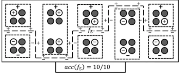
Fig. 3 provides an example of how forcing a subsequent function to learn all the incorrect instances can increase its complexity. In Fig. 3, there are 10 separate areas of instan-ces. In each of these 10 areas, the previous functions (not shown) predicted the correct labels for 3/4 instances leaving a single incorrect instance in each area. The decision bound-ary required for a subsequent function (f5) to learn to label

all the incorrect instances correctly is shown. Specifically, thisf5 function predicts a label (þ) for instances above the

line and () for instances below the line (surrounding squares) achieving perfect accuracy on the previously incor-rect instances from all areas (10/10 corincor-rect). However, f5

requires a more complex and convoluted decision boundary than the functions in Figs. 1 and 2. The chance off5

overfit-ting is further increased because it only has access to a lim-ited amount of the training data and those instances are widely separated. As shown in Figs. 1 and 2, when the incorrect instances are not representative of their areas, the predictive accuracy of the subsequent function tends to suf-fer contributing to overfitting.

Overall, learning subsequent functions on widely sepa-rated instances requires functions with additional complexity. These complex functions achieve high accuracy on the train-ing data, but reduced predictive accuracy when those instances are not representative—resulting in the function overfitting. This overfitting is propagated into the final deci-sion since that function contributes to the weighted vote. Fur-thermore, functions with higher training accuracy get a larger weight. In this way, a function that overfits and achieves high training accuracy contributes more to the final decision than

Fig. 2. Example of how filtering affects subsequent functions given areas with label noise (C3-C4). The square instances are those with label noise. Theaccdenote the weighted accuracy for initial and subsequent functions (f3andf4).Theþ/symbols denote the actual labels, the sur-rounding squares denote the predicted labels for the functions, the grey circles are unused correct instances, and the‘symbol are a wrong pre-dicted label. (a) After learning the initial function, (b) after learning a sub-sequent function, and (c) boosting prediction.

Fig. 3. Example of increased complexity for a subsequent function learned on all the incorrect instances (f5Þ. Theþ/symbols denote the actual labels of the incorrect instances, the surrounding squares denote the predicted labels for the function, and the grey circles denote the unused correct instances.

(7)

another function. Unfortunately, simply restricting function complexity (e.g., through regularization [6]) is not an effective solution because such functions still have trouble accommo-dating all the difficult and widely separated training data (due to the same filtering discussed previously and shown in Figs. 1 and 2). These simple functions are likely to have low accuracy and contradictory predictions making their useful-ness to the final decision suspect.

Our solution to deal with function complexity is to break up the difficult and widely separated training data and learn a separate function with unrestricted complexity on each area. In this way, we reduce the likelihood of overfit-ting without restricoverfit-ting function complexity.

As a final note, some might argue that previous sec-tions have solusec-tions in direct opposition, namely, that the solution to Section 3.1.1 looks at the training data together, while the solution to Section 3.1.2 looks at that data separately. Instead, our solutions focus on different aspects of the training data: Section 3.1.2 tries to break up the training data into different areas, while Section 3.1.1 looks at both the correct and incorrect data in the same area. This allows for a more comprehensive, combined solution to the boosting problem, without the need to bal-ance individual solutions against one another.

3.2 Cluster-Based Boosting Solution

Here we further discuss our cluster-based boosting solu-tion. The main strategy for CBB is to incorporate clusters created on the training data directly into the boosting pro-cess using these clusters and the initial function to learn the subsequent functions. First, the clusters created pro-vide additional structure for the subsequent functions since these clusters include both correct and incorrect instances from previous functions. This structure helps to mitigate the filtering problem in subsequent functions pre-viously discussed in Section 3.1.1. Next, these clusters are designed to break up the training data into different areas since each cluster encapsulates only instances with a high degree of similarity. These separate areas help to mitigate overfitting in subsequent functions as in Section 3.1.2.

3.2.1 Cluster Creation

Our CBB solution is based on unsupervised clustering that tries to decompose or partition the training data into clus-ters where the member instances in a cluster are similar to each other and as different as possible from members in other clusters [30]. There are many different strategies for creating clusters on the training data. Probably the most popular strategy for clustering isk-Means (centroid-based) that assigns training data to the cluster to minimize the dis-tance between each member and the cluster center [31]. The CBB solution uses k-Means in this paper to establish that clustering can improve boosting in a general way. In the future work, we discuss further howotherclustering strate-gies can be used with the CBB solution.

The goal for k-Means clustering is to assign each instance to the cluster that minimizes the following objec-tive function [31]: Xk c¼1 X xi2pc jjximcjj2 (1)

wherexi is the instance,pc is the cluster,mc is the cluster centroid, and norm squared is the distance between the member instance and the cluster center. (Fork-Means, dis-tance and similarity are inversely proportional with zero distance corresponding to perfect similarity.) This objective function is difficult to solve precisely andk-Means cluster-ing usually employs an iterative method where cluster assignments are updated until the distance between the members is minimized [31]. As expected for clustering, min-imizing this objective function results in compact clusters whose centroids are as close as possible to members, but as far as possible from other centroids.

The principal advantage for k-Means clustering is that clusters are created based on instance similarity without

using the instance labels.

First, by finding compact clusters on the training data,

k-Means more easily identifies areas with similar instances than SL functions, whose primary motivation is finding a decision boundary that maximizes accuracy. As shown in Fig. 1, to maximize accuracy on the training data,f1predicts

the same label for widely separated areas (e.g., A1 and B2). On the other hand,k-Means with four clusters will encapsu-late each area within a cluster.

Second, by creating the clusters independently of the labels, k-Means provides additional structure—cluster membership—on the training data when the labels are fac-tored in. Suppose that each area in Fig. 1 is encapsulated in a separate cluster. When we evaluate the member labels, we observe that clusters for B1 and B2 have the same (homoge-nous) labels whereas A1 and A2 have multiple, different (heterogeneous) labels. The homogenous clusters are rela-tively easy for a function since it can predict the same label for all members. On the other hand, heterogeneous clusters are more difficult since the function must learn a decision boundary that can separate members with different labels in close proximity.

Overall, both homogenous and heterogeneous clusters provide additional structure on the training data that can be useful for the boosting process. As previously shown, learning a subsequent function on label noise (in an other-wise homogenous cluster) leads to filtering and reduced predictive accuracy. Alternatively, learning a subsequent function directly on a troublesome area (in a heteroge-neous cluster) actually reduces filtering and function complexity since the function can focus exclusively on the troublesome instances and does not have to learn widely separated instances. As discussed in Section 3.2.2, the CBB solution leverages this additional structure to selec-tively learn subsequent functions.

The principal limitation fork-Means clustering is that the number of clusters used (the k) must be specified beforehand. Our CBB solution addresses the limitation in

k-Means clustering by using a modified version called

X-Means that learns the appropriate number of clusters automatically [32].X-Means starts with the set of clusters from a small k and then dynamically increases k as long as it lowers the Bayesian Information Criterion (BIC) [33] in the new set of clusters:

(8)

where xis all the training data in cluster pc ands^2 is the same as the inner summation in (1). The value of k when BIC is minimal is thus considered the optimal number of clusters for the data set. Note that the BIC metric rewards sets of clusters containing similar members, while penaliz-ing clusters that are too small. In this way, the BIC encour-ages cluster compactness while discouraging clusters too small to encapsulate meaningful areas.

3.2.2 Learning Subsequent Functions

As alluded to earlier, CBB uses a modified boosting process that learns subsequent functions selectively on the clusters. CBB consider four different cluster types based on two inde-pendent factors: cluster membership (heterogeneous and homogenous) and previous function accuracy (prospering and struggling). As described in Section 3.2.1, clusters are cre-ated independently of the previous functions. Evaluating the member labels gives an estimate for how difficult those mem-bers will be for subsequent functions. For example, memmem-bers that are similar and yet have different (heterogeneous) labels could indicate a difficult decision boundary (e.g., from trou-blesome areas) requiring high-eta boosting. This estimate is useful for selective boosting early on when the previous func-tions are prone to misusing the training data as described in Section 3.1.1. However, previous function accuracy measured on the cluster members also gives a useful estimate for selec-tive boosting. Whereas the cluster membership isstatic, based on clusters and labels, the previous function accuracy dynami-cally reflects mastery of the functions on the training data. Considering the previous example of members that are simi-lar and yet have different labels, this estimate is useful for checking whether the initial function could actually learn the complex decision boundary. This estimate is also useful later on during boosting to avoid overfitting (Section 3.1.2). There-fore, taken together, the cluster membership and previous function accuracy provide CBB with a more representative view on how the functions are doing than using only cluster membership. In turn, this provides more options for selective boosting as described below and summarized in Table 1. Note that these cluster types are given in a descending order of difficulty for the functions.

Heterogeneous struggling. The cluster contains mem-bers withdifferentlabels and previous functions strug-gleto predict the correct labels. Since such a cluster generally contains troublesome training data and pre-vious functions have been struggling, CBB uses boosting with a high learning rate (high-eta boosting) on this type—learning subsequent functions focusing on incorrect members until accuracy improves.

Heterogeneous prospering. The cluster contains mem-bers withdifferentlabels, but previous functions are still able to predict thecorrect label for most of the members. Since such data is difficult and (based on margin theory, Section 2.1), boosting can still make improvements by refining the final decision bound-ary, CBB uses boosting with a low learning rate (low-eta boosting) on this type—learning fewer sub-sequent functions focusing on incorrect members. Homogenous struggling. The cluster contains members

with predominately asingle label, but the previous functionsstruggle to predict the correct labels. This type can happen when the previous functions sacri-fice these members focusing instead on learning other areas of the training data to achieve the highest accuracy. Since this type is easy for a function to pre-dict (simply by prepre-dicting the majority label), CBB learns a single, subsequent function on all members without boosting on incorrect members.

Homogenous prospering. The cluster contains members with predominately asingle label and the previous functions already predict thecorrectlabel for most of the members. CBB does not learn any subsequent functions on this type to prevent those functions from learning the label noise as discussed in Section 3.1. Referring back to Figs. 1 and 2, we show how CBB utilizes these cluster types for selective boosting. For Fig. 1, A1 and A2 are the most difficult HES type since each contains mem-ber data with different labels andf1 is struggling on them.

B1 and B2 are the least difficult HOP type since each contains data with the same label andf1 is doing well. On this data

set, CBB refines the decision boundary by high-eta boosting on A1 and A2, while leaving B1 and B2 alone. If a more complex function is used, that gets additional instances in A1-A2 correct, these clusters could be HEP instead resulting in low-eta boosting (B1 and B2 would be unchanged). For Fig. 2, all the clusters are considered to be HOP and left alone allowing CBB to avoid fitting label noise. Using a more complex function does not change these clusters.

The four cluster types are computed using two separate metrics. First, the localized estimate (LE) metric is used to decide whether a cluster is struggling or prospering:

LEðpcÞ ¼ prospering_struggling_otherwiseif accðF;pcÞ 1d1

(3) where acc F;ð pcÞ is the accuracy of the previous functions evaluated only on the cluster members andd1 is a tunable

parameter on the range0:1d10:3. This range is sensible

because (1) a smallerd1(<0.1) would render the typing too

strict such that almost all clusters would fall into the strug-gling category and (2) a larger d1 (>0.3) would probably

allow too many “borderline struggling” clusters to be con-sidered prospering.1 Second, the minority label estimate

TABLE 1

Summary of Properties for the Cluster Types in CBB

Type Cluster Structure Prev. Functions Boosting Action HES Heterogeneous Struggling High Learn Rate HEP Heterogeneous Prospering Low Learn Rate HOS Homogeneous Struggling Single Function

HOP Homogeneous Prospering Nothing

The Type is used in the CBB approach in Section 3.3. Structure is described in Section 3.1, while previous functions and boosting action are described in the bullets in Section 3.2.

1. In general, this parameter uses a range to accommodate accuracy variations based on the type of function used. More complex func-tions, say, from neural networks, need a higher threshold for prosper-ing since they generally return a higher accuracy than functions from decision trees. In machine learning parlance, functions with higher built-in regularization, such as decision trees, should have lower threshold values for prospering.

(9)

(MLE) is used to decide whether a cluster is homogenous or heterogeneous:

MLEðpcÞ ¼ homogenous_{heterogeneous}if minority_otherwiseðpcÞ < d2

(4) whereminorityðpcÞis the minority label percentage on the cluster members andd2is a tunable parameter on the range

0:2d20:4.2 This parameter uses a range to

accommo-date data sets with varying label distributions. Data sets with a larger skew towards the majority label need a corre-spondingly smaller threshold.

Last, CBB computes the weighted vote for a function using the method adapted from Opelt et al. [34]:

vote fð Þ ¼t hln 1_""t t

(5) whereftis the function,his thelearning rateused to control the update of the weights for the incorrect instances, and"t is the weighted error on the member data. As usual for boosting, this vote is also used as the basis for updating instance weights in the boosting probability distribution.

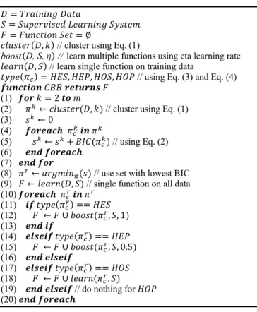
3.3 Cluster-Based Boosting Approach

We now discuss our approach for the CBB solution with pseudocode provided in Fig. 4. First, the training data is bro-ken into sets of clusters with varyingkwhere each set of clus-ters minimizes the objective function from (1) (Lines 1-7). During this process, CBB computes the BIC for the set of

clusters (Line 5). Second, CBB chooses the set of clusters with the lowest BIC (Line 8). Third, CBB learns the initial function using all the training data (Line 9).

After clustering, CBB performs selective boosting based on the cluster type (Lines 10-20). The cluster type (cf., Table 1) is computed using the localized estimate metric from (3) and the minority label (MLE) metric from (4). If the cluster is Heterogeneous Struggling (HES), high-eta boost-ing has a learnboost-ing rate on the high end for AdaBoost (h¼1) (Lines 11-13). Otherwise, if the cluster is Heterogeneous Prospering (HEP), low-eta boosting has a learning rate on the low end for AdaBoost (h¼0:5) (Lines 14-17). Otherwise, if the cluster is Homogeneous Struggling (HES), a single function is learned without boosting (Lines 18-20). No func-tions are learned if the cluster is Homogeneous Prospering (HEP) to avoid learning label noise.

After selective boosting, the set of functions is assigned the weighted vote based on (5) and used to predict the labels for a new instance. There are two different ways that these subsequent functions can be used:restrictedand unre-stricted. Both of course would count the initial function in the voting. Restricted only counts the subsequent functions learned on the cluster to which the new instance would be assigned and disregards votes from other clusters. Unre-stricted counts the votes from subsequent functions learned from all the clusters. We use restricted CBB in the rest of this paper because it is more consistent with the proposed selective boosting on each cluster.

4 I

MPLEMENTATION AND

R

ESULTS

In this section, we start by describing the experimental setup including the data sets, supervised learning systems, and the cross-validation process used to evaluate the predictive accuracy. We then discuss the results for three studies used to establish the effectiveness of our proposed cluster-based boosting in Sections 4.1-4.4. To summarize, the first study compares CBB to the most popular boosting algorithm: Ada-Boost [4]. The second study compares CBB to an existing algorithm that uses clusters to improve boosting: Prune-Boost [17]. In Section 4.3, we discuss the clusters created by CBB in more detail to better understand tendencies and behaviors of CBB. The third study compares CBB to two reg-ularized boosting algorithms that use selective boosting without clusters: BrownBoost [25] and AdaBoostKL[26].

For all studies, we use 20 different benchmark data sets from the UCI machine learning repository [35]. Based on previously reported results [35], these benchmark data sets have a range of difficulty for the SL systems. These data sets also contain varying amounts of label noise and trouble-some areas. Additionally, all of these data sets have binary labels. We chose to use binary data sets to demonstrate the benefits of using CBB on the most common supervised learning task. The only change required to the CBB approach to support nonbinary labels would be updatingk (Line 1, Fig. 4) to the number of labels andmk.

Next, we consider three widely studied SL systems in the results below: multi-layer perceptrons (MLP), support vec-tor machines (SVM), decision trees (TREE). We chose these three SL systems because they use very different methods for learning and, thus, produce functions with varying

Fig. 4 CBB approach pseudocode.

2. The difference in range ford1 andd2 is actually the same given that the maximum training accuracy is 100 precent and the maximum minority label is 50 precent, respectively for LE and MLE, so both are off by 10 precent: 90 precent is the upperbound in LE and 40 precent in MLE.

(10)

complexity allowing us to assess and analyze our approaches more comprehensively. Briefly, MLPs itera-tively update the weights on a complex network of intercon-nected nodes until the network predicts the correct labels for the training data. SVMs use a kernel to map the training data into a high-dimensional feature space where the train-ing data with different labels are linearly separable. TREEs recursively identify the feature that best splits the training data into groups where instances in the same group have the same label.

Note that none of these SL systems are intrinsically superior to the others in terms of predictive accuracy. In general terms, MLPs functions are probably the most complex, followed by SVMs, followed by TREEs. Func-tion complexity can increase predictive accuracy. On the other hand, TREEs with post-pruning are probably the most resistant to overfitting, followed by SVMs with soft margins, followed by MLPs. Overfitting can reduce pre-dictive accuracy. Interested readers should consult [6] for more details on these SL systems.

We use the Java implementations for all SL systems from the Weka library with parameters based on Hall et al. [36]. We also use the Weka implementation for both AdaBoost and k-Means clustering with m¼10 (Fig. 4, Line 1). The PruneBoost implementation is based on the pseudocode in Kim et al. [17] using the samek-Means clustering as CBB.

Finally, we use 10-fold cross-validation to measure the predictive accuracy for the results reported below. The pur-pose of cross-validation is to reduce variance in the predic-tive accuracy [37]. In 10-fold cross-validation, the instances in the data set are randomly divided into 10 separate folds of approximately equal size. Next, cross-validation uses an iterative process to measure the predictive accuracy. During the first iteration, the instances in the first fold are used as the test data, while all instances in the remaining folds are used as the training data. Cross-validation then runs each pair of algorithms in the study on the training data and evaluates their predictive accuracy on the test data. This iterative process is repeated 10 times with each fold used, in turn, as the test data, while the remaining folds are used as the training data. The final predictive accuracy reported is measured by averaging the accuracy on all 10 validation folds. Additionally, the statistical significance reported is measured by using a paired t-test on the folds for both algorithms as recommended in Raeder et al. [37].

4.1 CBB versus AdaBoost: Is Cluster-Based Better?

Here we compare CBB to AdaBoost [4], which is the most popular boosting algorithm in existence to investigate the impact of using clusters in boosting. The CBB parameters for the localized estimate metric (d1in (3)) and the minority

label estimate metric (d2in (4)) are fine-tuned on each data

set. In the interest of fairness, both are run on exactly the sametraining and test data. The same SL system configura-tion is used for both algorithms.

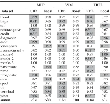
Table 2 provides the predictive accuracy for CBB and AdaBoost on the benchmark data sets using all three SL sys-tems. As shown, CBB has an advantage using all SL systems with a more pronounced advantage using SVM and TREE. On several data sets, this advantage is statistically significant using at-test on the validation folds.

In general, CBB achieves superior predictive accuracy on seven data sets using MLP (3 sig.), 11 data sets using SVM (2 sig.), and 11 data sets using TREE (4 sig.) com-pared to AdaBoost, which achieves superior accuracy on five data sets using MLP, one data sets using SVM, and six data sets for TREE (3 sig.). Furthermore, there are 12 data sets where CBB achieves higher accuracy for two or three of the SL systems, but only two data sets where AdaBoost achieves the same.

To better explain our results, we examine the source of the improved accuracy for CBB. After both CBB and AdaBoost finish predicting the labels for all the new instan-ces, we break these new instances down by CBB cluster type and compute the accuracy for each type.3 _{We found}

that the source of the improved accuracy for CBB is gener-ally the result of predictions on HES and HEP clusters: seven versus three using MLP on HES, six versus three using SVM on HEP, and nine versus four using TREE on HEP. CBB also achieves improved accuracy using SVM on HOP: six versus three. Taken together, these results support the effectiveness of our CBB selective boosting both in deciding when to boost on the clusters (HES and HEP) to address troublesome areas and when to refrain from boost-ing (HOP) to address label noise.

In summary, CBB leverages selective boosting on the clusters to achieve superior predictive accuracy compared to AdaBoost. These results on multiple, different types of clusters support our previous claim (cf., Section 3.2) that CBB helps address problems resulting from boosting on all the training data.

We have established that CBB achieves generally superior predictive accuracy to AdaBoost on benchmark data sets. However, real-world applications must consider additional

TABLE 2

Predictive Accuracy for CBB and AdaBoost

Data set

MLP SVM TREE CBB Boost CBB Boost CBB Boost

blood 0.79 0.78 0.77 0.77 0.78 0.77 bupa 0.71 0.65 0.72 0.67 0.70 0.67 car 1.00 1.00 0.99 0.99 0.96 0.99 contraceptive 0.72 0.69 0.69 0.69 0.70 0.67 credit 0.86 0.84 0.86 0.82 0.86 0.84 diagnostic 0.97 0.97 0.98 0.96 0.95 0.96 ecoli 0.99 0.98 0.99 0.99 0.99 0.98 ionosphere 0.91 0.92 0.91 0.88 0.90 0.93 mammography 0.82 0.82 0.81 0.80 0.82 0.79 monks-1 1.00 1.00 1.00 1.00 0.99 1.00 monks-2 1.00 1.00 1.00 1.00 0.68 0.56 monks-3 1.00 1.00 1.00 1.00 1.00 1.00 parkinsons 0.91 0.94 0.91 0.88 0.92 0.90 pima 0.77 0.77 0.77 0.77 0.75 0.71 prognostic 0.78 0.76 0.77 0.73 0.77 0.82 sonar 0.82 0.83 0.82 0.84 0.80 0.73 spect 0.81 0.81 0.82 0.81 0.82 0.82 tic 0.97 0.98 1.00 0.99 0.94 0.96 vertebral 0.83 0.84 0.85 0.82 0.82 0.82 yeast 0.66 0.65 0.66 0.64 0.68 0.61 summ. 7(3) 5(0) 11(2) 1(0) 11(4) 6(3)

Grey cells denote higher accuracy with’s denoting significantly higher (t-test withfor p0.1,for p0.05,for p0.01)

(11)

factors such as the impact of class imbalance. The initial results for CBB with class imbalance are promising. We con-sidered the four benchmark data sets with class imbalance where the minority label is found in 25 percent or less of the training data (spect 21 percent, blood 24 percent, prognostic 24 percent, and parkinsons 25 percent). CBB achieved higher predictive accuracy using two or more SL systems for all except spect, where it achieved higher accuracy only using SVM. While promising, these results still required fine-tun-ing the minority label estimate for those data sets. Addition-ally, automatically setting CBB parameters could result in scalability issues for CBB on large data sets. These issues will be investigated in our future work.

4.2 CBB versus PruneBoost: When to Use Clusters?

Here we compare CBB to PruneBoost that also uses clusters to improve boosting [17]. As previously, both are run on the exact same training data, test data, and SL system. For fair-ness, the distance threshold for PruneBoost is also fine-tuned on each of the benchmark data sets. As in [17], Prune-Boost uses withk¼20for all data sets.

Table 3 provides the predictive accuracy for CBB and Pru-neBoost on the benchmark data sets using all three SL sys-tems. As shown,CBB has a pronounced advantage using all three SL systems. In general, CBB achieves superior predictive accuracy on nine data sets using MLP (3 sig.), 12 data sets using SVM (5 sig.), and 10 data sets using TREE (3 sig.). Pru-neBoost achieves superior accuracy on only four data sets for MLP, one data set for SVM, and five data sets for TREE (2 sig.). Furthermore, there are 11 data sets where CBB achieves higher accuracy on two or three of the SL systems consid-ered, but only two data sets where PruneBoost does.

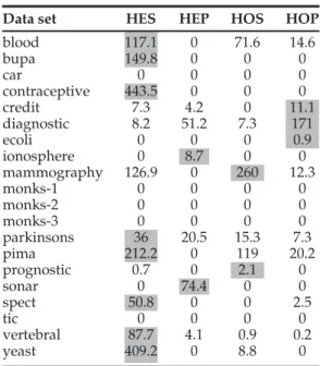
To explain the difference in performance, we examine which instances are removed from the training data by Pru-neBoost. To do so, after both CBB and PruneBoost finish predicting the labels for all the new instances, we break these new instances down by CBB cluster type and look at the number of instances PruneBoost removes from each type. PruneBoost removes some training data whose labels do not match the majority from the relative easy clusters: homogeneous struggling (HOS) and homogeneous prosper-ing (HOP). In an otherwise homogenous cluster, instances whose labels do not match the majority are more likely to be noise. As previously discussed, removing these instances before boosting can improve the predictive accuracy for boosting. However, the training data PruneBoost removes from a more difficult cluster type gives a very different pic-ture. As shown in Table 4, with a distance threshold of 0.1, PruneBoost removes relatively more training data instances from the most difficult HES clusters. By aggressively prun-ing instances from these clusters, PruneBoost removes criti-cal information about troublesome areas that are already difficult for boosting to learn. As a result, PruneBoost has a difficult time predicting the correct label for new instances in these clusters.

In summary, CBB selective boosting on the clusters achieves superior predictive accuracy compared to Prune-Boost. CBB uses selective boosting separately on the clus-ters, but factors in all the member instances. In this way, CBB does not risk removing critical information from clus-ters that can damage the boosting process.

4.3 CBB Clusters: What Types are Used?

Here we investigate the clusters that CBB creates on the training data in greater detail. First, the number of clus-ters that CBB creates is the same regardless of the SL system, but the cluster types vary depending on the SL

TABLE 3

Predictive Accuracy for CBB and PruneBoost

Data set

MLP SVM TREE CBB Prune CBB Prune CBB Prune

blood 0.79 0.78 D2 0.77 0.77 D2 0.78 0.77 D2 bupa 0.71 0.61 D1 0.72 0.62 D1 0.70 0.67 D1 car 1.00 1.00 D1 0.99 0.99 D1 0.96 0.98 D1 contra. 0.72 0.64 D1 0.69 0.63 D1 0.70 0.64 D1 credit 0.86 0.84 D2 0.86 0.82 D1 0.86 0.84 D2 diagnostic 0.97 0.98 D1 0.98 0.97 D1 0.95 0.95 D1 ecoli 0.99 0.98 D2 0.99 0.98 D1 0.99 0.99 D1 ionosphere 0.91 0.91 D1 0.91 0.88 D1 0.90 0.93 D1 mamm. 0.82 0.80 D1 0.81 0.81 D1 0.82 0.80 D1 monks-1 1.00 1.00 D1 1.00 1.00 D1 0.99 1.00 D1 monks-2 1.00 1.00 D1 1.00 1.00 D1 0.68 0.59 D1 monks-3 1.00 1.00 D1 1.00 1.00 D1 1.00 1.00 D1 parkinsons 0.91 0.91 D1 0.91 0.88 D1 0.92 0.89 D1 pima 0.77 0.76 D1 0.77 0.76 D1 0.75 0.73 D1 prognostic 0.78 0.78 D3 0.77 0.77 D3 0.77 0.77 D3 sonar 0.82 0.84 D1 0.82 0.84 D1 0.80 0.83 D1 spect 0.81 0.83 D1 0.82 0.79 D1 0.82 0.81 D1 tic 0.97 0.98 D1 1.00 0.99 D1 0.94 0.97 D1 vertebral 0.83 0.82 D2 0.85 0.81 D2 0.82 0.82 D2 yeast 0.66 0.63 D1 0.66 0.61 D1 0.68 0.62 D1

summ. 9(3) 4(0) N/A 12(5) 1(0) N/A 10(5) 5(2) N/A

Grey cells denote higher accuracy with’s denoting significantly higher (t-test withfor p0.1,for p0.05,for p0.01). The Ds denote fine-tuned distance threshold for PruneBoost (D1¼0.1, D2¼0.2, D3¼0.3).

TABLE 4

Instances Removed for PruneBoost by Cluster Type

Data set HES HEP HOS HOP

blood 117.1 0 71.6 14.6 bupa 149.8 0 0 0 car 0 0 0 0 contraceptive 443.5 0 0 0 credit 7.3 4.2 0 11.1 diagnostic 8.2 51.2 7.3 171 ecoli 0 0 0 0.9 ionosphere 0 8.7 0 0 mammography 126.9 0 260 12.3 monks-1 0 0 0 0 monks-2 0 0 0 0 monks-3 0 0 0 0 parkinsons 36 20.5 15.3 7.3 pima 212.2 0 119 20.2 prognostic 0.7 0 2.1 0 sonar 0 74.4 0 0 spect 50.8 0 0 2.5 tic 0 0 0 0 vertebral 87.7 4.1 0.9 0.2 yeast 409.2 0 8.8 0

Grey cells denote the cluster type with the largest number of instances removed (averaged over validation folds).

(12)

system (cf., Section 3.3). Second, the number of clusters reported is not always an integer. CBB creates a separate set of clusters for each validation fold and the results are averaged together.

Tables 5, 6 and 7 provide the number of clusters and clus-ter types for CBB on the benchmark data sets using MLP (Table 5), SVM (Table 6), and TREE (Table 7). The number

of clusters is reported along with the percentage breakdown for all four cluster types (cf., Section 3.2.2).

First, the data sets vary considerably in terms of the pre-dominant or favored cluster type used. In fact, there are one or more data sets that favors each cluster type in all three tables. Additionally, based on the number of clusters and percentage breakdown, the majority of the data sets use clusters with multiple types. These results make sense given that the benchmark data sets have a high degree of diversity (cf., Section 4 and [35]). In other words, CBB found clusters with different types not only between data sets, but on the same data set.

Second, although percentages vary, we observe patterns in the favored cluster types across SL systems for different data sets. As an example, contraceptive-ionosphere favor HOP clusters in Tables 5, 6 and 7 while sonar, tic, and verte-bral favor HEP. As previously discussed (Lines 1–7 in Fig. 4), CBB creates the clusters using an unsupervised clus-tering algorithm that operates independently of the SL sys-tem. Then, CBB uses the SL system to help compute the cluster type using the localized estimate metric (3) and minority label metric (4). Now, these SL systems produce functions with varying complexity (cf., Section 4) and prop-erties. The presence of these patterns, despite functions with varying complexity, suggests that selective boosting on the set of clusters is effective across multiple SL systems and on data sets that favor each cluster type.

4.4 CBB versus Regularized Boosting

Here we compare CBB with two regularized boosting algo-rithms: BrownBoost [25] and AdaBoostKL [26] described in

Section 2.3. We fine-tune both thet parameter for Brown-Boost and thebparameter for AdaBoostKL. For both

param-eters, we consider values of 0.25, 0.5, and 0.75 based on the

TABLE 7

Number of Clusters and Types for CBB with TREE

Data set

Parameters Cluster Type

d1 d2 Clusters HES HEP HOS HOP blood 0.1 0.3 6.3 29% 0% 56% 16% bupa 0.3 0.2 4 0% 100% 0% 0% car 0.1 0.2 6.7 10% 69% 0% 21% contraceptive 0.3 0.2 6.1 5% 95% 0% 0% credit 0.1 0.4 3.8 5% 0% 42% 53% diagnostic 0.1 0.2 5.3 0% 25% 0% 75% ecoli 0.1 0.2 2.9 0% 10% 0% 90% ionosphere 0.1 0.3 3.4 0% 18% 0% 82% mammography 0.1 0.2 5.2 29% 0% 63% 8% monks-1 0.2 0.4 3.1 0% 97% 0% 3% monks-2 0.1 0.4 3.1 0% 0% 100% 0% monks-3 0.1 0.2 3.1 0% 100% 0% 0% parkinsons 0.2 0.2 3.5 0% 51% 0% 49% pima 0.1 0.4 5.3 60% 2% 32% 6% prognostic 0.1 0.3 3 7% 23% 10% 60% sonar 0.1 0.2 3 0% 100% 0% 0% spect 0.2 0.2 3.4 9% 29% 3% 59% tic 0.2 0.2 3.7 0% 97% 0% 3% vertebral 0.3 0.2 3.3 0% 61% 0% 39% yeast 0.3 0.3 6.8 13% 59% 0% 28%

Parameters denote the fine-tuned parameters for CBB. Clusters denote the average number of clusters used. Cluster type denotes the percentage of cluster type for each data set. Grey cells denote the favored cluster type.

TABLE 5

Number of Clusters and Types for CBB with MLP

Data set

d1 d2 Clusters HES HEP HOS HOP blood 0.1 0.2 6.3 51% 0% 33% 16% bupa 0.1 0.2 4 100% 0% 0% 0% car 0.1 0.2 6.7 0% 79% 0% 21% contraceptive 0.3 0.4 6.1 7% 33% 2% 59% credit 0.1 0.3 3.8 16% 5% 11% 68% diagnostic 0.1 0.4 5.3 2% 0% 2% 96% ecoli 0.1 0.2 2.9 0% 10% 0% 90% ionosphere 0.1 0.2 3.4 0% 35% 0% 65% mammography 0.2 0.2 5.2 29% 0% 4% 67% monks-1 0.1 0.2 3.1 0% 100% 0% 0% monks-2 0.1 0.2 3.1 0% 100% 0% 0% monks-3 0.1 0.2 3.1 0% 100% 0% 0% parkinsons 0.1 0.2 3.5 23% 29% 9% 40% pima 0.2 0.2 5.3 70% 11% 0% 19% prognostic 0.2 0.4 3 0% 0% 3% 97% sonar 0.1 0.2 3 0% 100% 0% 0% spect 0.1 0.4 3.4 9% 0% 26% 65% tic 0.1 0.2 3.7 0% 97% 0% 3% vertebral 0.1 0.3 3.7 0% 81% 0% 19%

TABLE 6

Number of Clusters and Types for CBB with SVM

Data set

d1 d2 Clusters HES HEP HOS HOP blood 0.2 0.3 6.3 29% 0% 21% 51% bupa 0.3 0.2 4 40% 60% 0% 0% car 0.1 0.2 6.7 0% 79% 0% 21% contraceptive 0.3 0.4 6.1 13% 26% 7% 54% credit 0.2 0.3 3.8 0% 21% 0% 79% diagnostic 0.1 0.4 5.3 0% 2% 0% 98% ecoli 0.1 0.2 2.9 0% 10% 0% 90% ionosphere 0.1 0.2 3.4 0% 35% 0% 65% mammography 0.1 0.3 5.2 21% 0% 77% 2% monks-1 0.1 0.2 3.1 0% 100% 0% 0% monks-2 0.1 0.2 3.1 0% 100% 0% 0% monks-3 0.1 0.2 3.1 0% 100% 0% 0% parkinsons 0.1 0.2 3.5 23% 29% 3% 46% pima 0.3 0.2 5.3 21% 60% 0% 19% prognostic 0.2 0.2 3 0% 60% 0% 40% sonar 0.1 0.2 3 0% 100% 0% 0% spect 0.1 0.3 3.4 24% 3% 3% 71% tic 0.1 0.2 3.7 0% 97% 0% 3% vertebral 0.3 0.2 3.3 0% 61% 0% 39% yeast 0.3 0.3 6.8 68% 4% 0% 28%

(13)

range given in Schapire & Freund [4]. The best results for each data set are reported in this section.

For completeness, we also provide results for all three using radial basis functions (RBF) considered in Sun et al. [26]. RBFs use a network of interconnected nodes similar to MLPs, but both the update procedure and the nodes used are radically different.

Tables 8 and 9 provide the predictive accuracy for CBB compared to BrownBoost and AdaBoostKL. As shown in

Table 8, CBB has a pronounced advantage compared BrownBoost using all four SL systems. CBB achieves supe-rior predictive accuracy on 12 data sets using MLP (5 sig.), 11 data sets using SVM (4 sig.), 15 data sets using TREE (7 sig.), and 11 using RBF (5 sig.). As shown in Table 9, CBB has the advantage using MLP, SVM, and RBF, while Ada-BoostKL has the advantage using TREE. CBB achieves

superior predictive accuracy on seven data sets using MLP (3 sig.), 11 data sets using SVM (1 sig.), four data sets using TREE (0 sig.), and 13 using RBF (5 sig.). On the other hand, AdaBoostKL achieves superior accuracy on three

data sets using MLP, three data sets using SVM (1 sig.), nine data sets using TREE (4 sig.), and two data sets using RBF (1 sig.).

The above results show that CBB has a performance advantage over both AdaBoostKLand BrownBoost. During

our investigation, we found three specific reasons explain-ing this advantage.

First, we found that the number of functions learned by BrownBoost was much lower than that used by conven-tional AdaBoost (recall that CBB uses AdaBoost). When averaged across all data sets, the number learned was 3 versus 7.75 using MLP, 3.53 versus 8.35 using SVM, 1.75 versus 9.56 using TREE, and 4.32 versus 9.29 using RBF. Furthermore, on many data sets, AdaBoost used the full

allotment of boosting iterations, while BrownBoost stopped after the initial function. Based on these results, BrownBoost seems to be stopping too early—consistent with Warmuth et al. [27] who also reported that BrownBoost stopped early. Second, we found that the sum of the weights learned by AdaBoostKL for the subsequent function was sometimes

lower than the weight for the initial function. The number of data sets where the subsequent functions had sufficient weight to contribute was nine using MLP, 11 using SVM, 17 using TREE, and only two using RBF. This means that the subsequent functions played no part predicting the label since the initial function had the dominant vote. Based on these results, AdaBoostKLmay be reducing the weights for

subsequent functions too aggressively for the subsequent functions to impact the final vote.

Third, we also found a direct link for AdaBoostKL

between performance (see Table 9) and the number of data sets where subsequent functions were used. AdaBoostKL

used subsequent functions most often for TREE where it achieved the best accuracy compared to CBB. On the other hand, subsequent functions were used least often for RBF where AdaBoostKL achieved, by far, the worst accuracy

compared to CBB. Indeed, AdaBoostKLis aggressively

selec-tive and subsequent functions contribute little; but when the initial function has low accuracy (TREE), AdaBoostKL is

more willing to use the subsequent functions.

In summary, CBB simplifies the boosting process by breaking up the training data into clusters containing similar instances. Selective boosting can then be used more precisely on the instances in the same cluster. This allows CBB selec-tive boosting to more easily distinguish between (1) instan-ces difficult for the initial function and (2) instaninstan-ces that genuinely have label noise. On the other hand, BrownBoost’s conservative behavior of stopping early makes sense since

TABLE 8

Predictive Accuracy for CBB and BrownBoost

Set MLP SVM TREE RBF CBB BB CBB BB CBB BB CBB BB blood 0.80 0.78 0.78 0.77 0.78 0.76 0.78 0.78 bupa 0.70 0.67 0.72 0.69 0.67 0.64 0.69 0.69 car 1.00 1.00 0.99 0.99 0.96 0.94 0.97 0.95 cont. 0.72 0.69 0.69 0.69 0.70 0.69 0.68 0.70 credit 0.87 0.86 0.87 0.85 0.86 0.86 0.86 0.86 diag. 0.97 0.95 0.98 0.98 0.95 0.94 0.98 0.97 ecoli 0.99 0.98 0.99 0.99 0.99 0.99 0.98 0.98 iono. 0.91 0.89 0.91 0.89 0.89 0.89 0.94 0.93 mamm. 0.82 0.82 0.82 0.81 0.82 0.82 0.81 0.82 mks-1 1.00 1.00 1.00 1.00 0.99 0.91 0.96 0.87 mks-2 1.00 1.00 1.00 1.00 0.68 0.59 0.71 0.78 mks-3 1.00 1.00 1.00 1.00 1.00 0.99 1.00 0.97 park. 0.92 0.88 0.94 0.86 0.90 0.83 0.90 0.82 pima 0.77 0.77 0.77 0.76 0.75 0.72 0.77 0.75 prog. 0.80 0.74 0.77 0.78 0.79 0.74 0.80 0.78 sonar 0.81 0.79 0.82 0.79 0.79 0.69 0.83 0.76 spect 0.81 0.80 0.82 0.78 0.84 0.77 0.85 0.82 tic 0.97 0.97 1.00 0.97 0.94 0.84 0.97 0.96 vert. 0.82 0.83 0.82 0.83 0.83 0.84 0.83 0.84 yeast 0.65 0.64 0.66 0.65 0.66 0.64 0.64 0.68 summ. 12(5) 1(0) 11(4) 2(0) 15(7) 1(0) 11(5) 5(2) Grey cells denote higher accuracy with’s denoting significantly higher (t-test withfor p0.1,for p0.05,for p0.01).

TABLE 9

Predictive Accuracy for CBB and AdaBoostKL

Set MLP SVM TREE RBF CBB KL CBB KL CBB KL CBB KL blood 0.80 0.78 0.78 0.77 0.78 0.77 0.78 0.78 bupa 0.70 0.59 0.72 0.66 0.67 0.72 0.69 0.62 car 1.00 1.00 0.99 0.99 0.96 0.98 0.97 0.95 cont. 0.72 0.69 0.69 0.68 0.70 0.70 0.68 0.68 credit 0.87 0.86 0.87 0.86 0.86 0.87 0.86 0.86 diag. 0.97 0.97 0.98 0.98 0.95 0.96 0.98 0.98 ecoli 0.99 0.99 0.99 0.98 0.99 0.99 0.98 0.98 iono. 0.91 0.92 0.91 0.89 0.89 0.94 0.94 0.93 mamm. 0.82 0.82 0.82 0.81 0.82 0.83 0.81 0.83 mks-1 1.00 1.00 1.00 1.00 0.99 0.99 0.96 0.89 mks-2 1.00 1.00 1.00 1.00 0.68 0.67 0.71 0.63 mks-3 1.00 1.00 1.00 1.00 1.00 0.99 1.00 0.97 park. 0.92 0.90 0.94 0.89 0.90 0.90 0.90 0.84 pima 0.77 0.77 0.77 0.77 0.75 0.75 0.77 0.76 prog. 0.80 0.79 0.77 0.80 0.79 0.79 0.80 0.75 sonar 0.81 0.85 0.82 0.85 0.79 0.81 0.83 0.78 spect 0.81 0.83 0.82 0.81 0.84 0.82 0.85 0.82 tic 0.97 0.97 1.00 0.99 0.94 0.96 0.97 0.96 vert. 0.82 0.85 0.82 0.85 0.83 0.85 0.83 0.78 yeast 0.65 0.64 0.66 0.64 0.66 0.66 0.64 0.65 summ. 7(3) 3(0) 11(1) 3(1) 4(0) 9(4) 13(5) 2(1) Grey cells denote higher accuracy with’s denoting significantly higher (t-test withfor p0.1,for p0.05,for p0.01).