Comparative Study of Classification Algorithms: Holdouts as Accuracy Estimation

e-ISSN: 2477-8079 This article has been accepted for publication in Cogito Smart

COMPARATIVE STUDY OF CLASSIFICATION

ALGORITHMS: HOLDOUTS AS ACCURACY

ESTIMATION

Debby E. Sondakh

Universitas Klabat, Jl. A. Mononutu Airmadidi Minahasa Utara, 0431-891035 Teknik Informatika Fakultas Ilmu Komputer Universitas Klabat

[email protected]

Abstrak

Penelitian ini bertujuan untuk mengukur dan membandingkan kinerja lima algoritma klasifikasi teks berbasis pembelajaran mesin, yaitu decision rules, decision tree, k-nearest neighbor (k-NN), naïve Bayes, dan Support Vector Machine (SVM), menggunakan dokumen teks multi-class. Perbandingan dilakukan pada efektifiatas algoritma, yaitu kemampuan untuk mengklasifikasi dokumen pada kategori yang tepat, menggunakan metode holdout atau percentage split. Ukuran efektifitas yang digunakan adalah precision, recall, F-measure, dan akurasi. Hasil eksperimen menunjukkan bahwa untuk algoritma naïve Bayes, semakin besar persentase dokumen pelatihan semakin tinggi akurasi model yang dihasilkan. Akurasi tertinggi naïve Bayes pada persentase 90/10, SVM pada 80/20, dan decision tree pada 70/30. Hasil eksperimen juga menunjukkan, algoritma naïve Bayes memiliki nilai efektifitas tertinggi di antara lima algoritma yang diuji, dan waktu membangun model klasiifikasi yang tercepat, yaitu 0.02 detik. Algoritma decision tree dapat mengklasifikasi dokumen teks dengan nilai akurasi yang lebih tinggi dibanding SVM, namun waktu membangun modelnya lebih lambat. Dalam hal waktu membangun model, k-NN adalah yang tercepat namun nilai akurasinya kurang.

Kata kunci- klasifikasi teks, dokumen multi-class, mesin learning

Abstract

This research aims to assess and compare the performance of five machine-learning algorithms for text classification namely decision rules, decision tree, k-nearest neighbor (k-NN), naïve Bayes, and Support Vector Machine (SVM). These five algorithms are compared for multi-class text document. The comparison was done in terms of effectiveness, the ability of multi-classifiers to classify the document in the right category, using holdout or percentage split method. Precision, recall, F-measure, and accuracy are the four effectiveness measurements that were applied. The experiment result shows that for Naïve Bayes algorithms, the greater the percentage of training documents, the higher the resulting model accuracy. Therefore, Naïve Bayes’ get the highest accuracy at percentage split of 90/10, while SVM is at 80/20 and decision tree is at 70/30. The result also shows, among the five algorithms Naïve Bayes classifiers has the highest effectiveness value, while the model building time is the shortest as well. It is 0.02 seconds. Decision tree can classify text with higher accuracy values rather than SVM, but slower in building the model. In terms of time to build the model, k-NN is the fastest but suffer in accuracy. Keywords- text classification, multi-class document, machine-learning approach

1. INTRODUCTION

Information retrieval system aims to obtain relevant information from a collection of large number of information. As the number of digital text documents spread over the internet

e-ISSN: 2477-8079 This article has been accepted for publication in Cogito Smart continues to grow every day, it triggers the need for a system that can organize the documents, and as well as make it easy for users to get the right and useful information. A number of algorithms and tools have been developed and implemented to retrieve information from large repositories.

Data mining provides solution to handle the rapid growth of data. Using data mining technique, the documents are grouping into classes in order to simplify the process of retrieving information from large set of data [1]. In data mining, there are two main approaches of grouping documents namely classification and clustering. Classification method groups the documents into fixed categories based on documents’ predefined labels. On the other hand, clustering method grouping the documents based on documents’ similarity.

Document classification is defined as grouping documents into one or more categories based on predefined label. Document classification starting with the learning process to determine the category of the document, is called supervised learning. This research investigated the text documents. Reference [2] and [3] defined text classification as a relation between two sets, set of documents, 𝑑 = (𝑑₁, 𝑑₂, ⋯ , 𝑑_𝑛) and set of categories 𝑐 = (𝑐₁, 𝑐₂, ⋯ , 𝑐_𝑚). 𝑑_𝑖 is i-th document to be classified. 𝑐_𝑗 is j-th predefined category for a document. 𝑛 is the number of documents to be classified, and 𝑚 is the total of predefined category in 𝑐. Text classification is the process of defining a Boolean value for each pair (𝑑_𝑗, 𝑐_𝑖) ∈ 𝐷 × 𝐶, where 𝐷 is the set of documents and 𝐶 is a set of predefined categories. Classification is about to approximate the classifier function (also called rule, hypothesis, or model):

𝑓: 𝐷 × 𝐶 → {𝑇, 𝐹}

The value 𝑇 (true) assigned to pair (𝑑_𝑗, 𝑐_𝑖) indicates that document 𝑑_𝑗 includes in category 𝑐_𝑖. Otherwise, the value 𝐹 indicates that document 𝑑_𝑗 is not a member of category 𝑐_𝑖.

Document is a sequence of words [4]. In information retrieval document is stored as set of words, also called vocabulary or feature set [5]. Vector Space Model is employed as document representation model. A document is an array of words, in the form of binary vector with value of 1 when a word present in the document or value of 0 for absences of a word. Each document is included in the vector space 𝑅|𝑉|, |𝑉| is the size of vocabularies 𝑉. For a collection of documents, called dataset, documents are represented as m x n matrix, where m is the number of documents and n is the words. Matrix element aijdenotes the occurrence of word j in document i which is represented as binary value.

There are two main approaches that can be applied for classifying document, i.e. rule-based approach and machine learning approach. In rule-rule-based approach, also called knowledge engineering, the rules that define the categories of documents are assigned manually by an expert. Then, the documents are grouped into categories that have been defined [2]. Using this method, rule-based classifier is able to produce an effective classification with good accuracy. However, its dependency on an expert to assign the rules manually becomes the main drawback. When the categories are about to change then the previous expert who defined the rules must be involved. Over all, this method requires high cost and takes time in classifying large number of documents [6]. This research aims to examine and compare text documents classification algorithms, specifically the machine learning based classification algorithms.

1.1 Machine Learning based Classification

To overcome the weaknesses of rule-based classifier, machine learning based approach is applied to perform classification. This method is also called inductive process or learner, in which the document classification is running automatically using the text label that have been defined first (predefined class). Machine learning based classifiers learn the characteristics of the set of documents, which have been classified into category 𝑐_𝑖. Using these characteristics, the inductive process is done to obtain new characteristics that the new documents must have to be included in a category. So, inductive process is a way of building the classifiers automatically

e-ISSN: 2477-8079 This article has been accepted for publication in Cogito Smart from set of documents that have been pre-classified. This method can overcome the problems of large document dataset, reducing labor cost, while the accuracy is comparable to the rules resulted from a supervisor.

A. Decision Tree

Decision rules using DNF rule to build a classifier for category 𝑐_𝑖. DNF rule is a conditional rule consists of disjunctive-conjunctive clause. This rule describes the requirements for the document to be classified into categories defined; ‘if and only if’ the document meets on of the criteria in DNF clauses. The rules in DNF clauses represent categories’ profile. Each single rule comprise of category’s name and the ‘dictionary’ (list of words included in that category). A collection of rules is the union of some single rule using logic operator “OR”. Decision rules will choose the rules whose scope is able to classify all the documents in training sets. Rules set can be simplified using heuristic without affecting the accuracy of resulting classifier.

Sebastiani in [2] explained, DNF rules are built in a bottom-up fashion, as follows: 1. Each training document 𝑑_𝑗 is 𝜂₁, … , 𝜂_𝑛 → 𝛾_𝑖 clause where 𝜂₁, … , 𝜂_𝑛 are the words contain

in document 𝑑_𝑗, and 𝛾_𝑖 is the category 𝑐_𝑖 when 𝑑_𝑗 satisfy the criteria of 𝑐_𝑖, otherwise it is 𝑐̅_𝑖. 2. Rules generalization. Simplifying the rules by removing the premise from clauses, or

merging clauses. Compactness of the rules is maximized while at the same time not affecting the ‘scope’ property of the classifier.

Pruning. The resulting DNF rules from step 1 may contain more than one DNF clauses, which able to classify documents in the same category (overfit). Pruning is done to ‘cut’ the unused clauses from the rule.

B. Decision Tree

Decision tree decomposes the data space into a hierarchical structure called tree. In textual data context, data space means the presence or absence of a word in the document. Decision tree classifier is a tree comprise of:

a. Internal nodes. Each internal node stores the attributes, i.e. collection of words, which will be compared with the words contained in a document.

b. Edge. Branches that come out of an internal node are the terms/conditions represent one attribute value.

c. Leaf. Leaf node is a category or class of documents.

Decision tree classifying document 𝑑_𝑗 by testing term weight of the internal nodes label contained in vector 𝑑̅_𝑗 recursively, until the document is classified at a leaf node. Label of the leaf node will be the document’s class. Decision tree classifiers are built in a top-down fashion [2]: 1. Starting from the root node, document 𝑑_𝑗 is tested whether it has the same label as the node’s

(category 𝑐_𝑖 or 𝑐̅_𝑖).

2. If the does not fit, select the 𝑘-th term (𝑡_𝑘), divide into classes of documents that have the same value as 𝑡_𝑘. Create a separated sub-tree for those classes.

3. Repeat step 2 in each sub-tree until a leaf node is formed. Leaf node will contain the documents in category 𝑐_𝑖.

The tree structure in decision tree algorithm is easy to understand and interpret, and the documents are classified based on their logical structure. On the contrary, this algorithm requires a long time to do the classification manually. When misclassification at the higher level occurs, it will affect the level below, and the possibility of overfit is high.

Sebastiani [2] explains, to reduce overfitting, several nodes can be trimmed (pruning), by withholding some of the attributes that are not used to build the tree. These attributes determine whether a leaf node will be pruned or not. The next step is comparing the class distribution in used attributes versus unused attributes. If the class distribution of the training documents used to construct the decision tree is different from the class distribution of the class distribution of the training documents retained for pruning, then the nodes are overfit to training documents and can be pruned.

e-ISSN: 2477-8079 This article has been accepted for publication in Cogito Smart C. k-Nearest Neighbor

In machine learning field k-nearest neighbor (k-NN) algorithm belongs to lazy learner group. Lazy learners, also called example-based classifier [2] or proximity-based classifier [7], do the classification task by utilizing the same existing category labels on the training documents with labels on the test documents.

k-NN starts by searching or determining the number of k nearest neighbor of the documents to be classified. Input parameter k indicates the number of document level to be considered in calculating document (𝑑_𝑗) classification function, 𝐶𝑆𝑉_𝑖(𝑑_𝑗). A document is compared with the neighbor classes, to calculate their similarity. Document 𝑑_𝑗 will become member of category 𝑐_𝑖 if there are k training documents that are similar to 𝑑_𝑗 in category 𝑐_𝑖. k-NN classification function is defined as follows:

𝐶𝑆𝑉𝑖(𝑑𝑗) = ∑ 𝑅𝑆𝑉(𝑑𝑗, 𝑑𝑧) ∙ ⟦Φ(𝑑𝑧, 𝑐𝑖)⟧ 𝑑𝑧∈𝑇𝑟𝑘(𝑑𝑗)

 _{𝑅𝑆𝑉(𝑑𝑗}, 𝑑𝑧) is a measure of relationship between testing document 𝑑𝑗 with training document 𝑑_𝑧.

 _{𝑇𝑟𝑘(𝑑𝑗)} is the set of 𝑘 testing document 𝑑_𝑧 to maximize the function 𝑅𝑆𝑉(𝑑_𝑗, 𝑑_𝑧). D. Naïve Bayes

Naïve Bayes is a kind of probabilistic classifier that utilize mixture model, a model that combine terms probability with category, to predict document category probability [7]. This approach define classification as the probability of document 𝑑_𝑗, which is represented as term vector 𝑑_𝑗= 〈𝑤_1𝑗, … , 𝑤_|𝑇|𝑗〉, belongs to category 𝑐_𝑖.

Document probability is calculated using the following equation:

𝑃

(𝑐_𝑖|𝑑⃗_𝑗)=

𝑃(𝑐𝑖)𝑃(𝑑⃗𝑗|𝑐𝑖)

𝑃(𝑑⃗𝑗)

where 𝑃(𝑑⃗_𝑗) is the probability of document 𝑑_𝑗 (randomly chosen), 𝑃(𝑐_𝑖) is the probability of a document to become classified in category 𝑐_𝑖.

The size of document vector 𝑑⃗_𝑗 may be large. Therefore, naïve Bayes applies word independence assumption. According to word independence assumption two different document vector coordinates are disjoint [2]. In other words, a term probability in a document does not depend on others. So, the presence of a word has no affect on others, so called ‘naïve’. Probabilistic classifier naïve Bayes is expressed in the following equation:

𝑃(𝑑⃗𝑗|𝑐𝑖) = ∏ 𝑃(𝑤𝑘𝑗|𝑐𝑖) |𝑇|

𝑘=1

There are two commonly used naïve Bayes variants, namely Multivariate Bernoulli and Multinomial Model.

a. Multivariate Bernoulli Model. This model using the term occurrence in document as the document feature. Term occurrence is represent as binary value, 1 and 0 (1 denoting presence and 0 absence of the term in the document). Term occurrence frequency is not taken into account for document classification modeling.

b. Multinomial Model. As oppose to multivariate model, this model considers the term occurrence frequency. Document is defined as ‘bag of words’, along with term frequency of each word. Classification modeling is conducted based on these occurrence frequencies in the document. Multinomial model has better performance compare with the other naïve Bayes variants [8, 9].

e-ISSN: 2477-8079 This article has been accepted for publication in Cogito Smart E. Support Vector Machine

Similar to regression-based classification, SVM represents documents as vectors. This approach aims to find a boundary, called decision surface or decision hyperplane, which separates two groups of vectors/classes. The system was trained using positive and negative samples from each category, and then calculated boundary between those categories. Documents are classified by first calculating their vectors and partition the vector space to determine where the document vector is located. The best decision hyperplane is selected from a set of decision hyperplane 𝜎₁, 𝜎₂, … , 𝜎_𝑛 in vector space |𝑇| dimension that separate the positive and negative training documents. The best decision hyperplane is the one with the widest margin [2, 7].

Figure 1. Contoh Support Vector Classifier [2]

Fig. 1 shows how SVM work. The cross (+) and circle () symbols represent two training document categories. Cross symbols for the positive ones and circle symbols otherwise. The lines represent decision hyperplanes, there are five decision hyperplanes on the example in Fig. 1. Box symbols are the support vectors, i.e. the documents whose distance against decision hyperplanes will be computed to determine the best hyperplane. 𝜎_𝑖 is the best one. Its normal distance against each training documents is the widest. Thus, 𝜎_𝑖become the maximum possible separation barrier..

1.2 Classifier Evaluation

Experimental approach was applied as document classifier evaluation method, to measure the effectiveness of the classifiers [2,6]. Classifier effectiveness describes the classifiers’ ability to classify a document in the right category. Three most often used methods to determine effectiveness applied in this study are precision, recall, and accuracy, based on probability technique. Table 1 shows the contingency table that is used to measure probability estimation for category 𝑐_𝑖.

To determine precision, recall, and accuracy must first begin by understanding if the classification of a document was a true positive (TP), false positive (FP), true negative (TN), and false negative (FN). TP means the documents being classified correctly as relating to a category. FP determined as documents that is related to the category incorrectly. FN describes documents that is not marked as related to a category but should be. TN means documents that should not be marked as being in a particular category.

TABLE I. CONTINGENCY TABLE FOR CATEGORY 𝑐_𝑖[2] Category 𝒄_𝒊 Expert Judgement YES NO Classifier Judgement YES 𝑻𝑷_𝒊 𝑭𝑷_𝒊 NO 𝑭𝑵_𝒊 𝑻𝑵_𝒊

e-ISSN: 2477-8079 This article has been accepted for publication in Cogito Smart a. Precision(𝝅). Precision, 𝜋, is defined as 𝑃(Φ̆(𝑑_{𝑥, 𝑐𝑖}) = 𝑇|Φ(𝑑_{𝑥, 𝑐𝑖}) = 𝑇), conditional probability of randomly chosen document 𝑑_𝑥 to be classified under category 𝑐_𝑖. Precision explains ability of the classifiers to place a document under the right category. The 𝑖𝑡ℎ document’s precision is calculated as:

𝜋𝑖 =_𝑇𝑃𝑇𝑃𝑖 𝑖+ 𝐹𝑃𝑖

b. Recall(𝝆). Recall, 𝜌, is determined as 𝑃(Φ(𝑑_𝑥, 𝑐_𝑖) = 𝑇|Φ̆(𝑑_𝑥, 𝑐_𝑖) = 𝑇), the probability of decision is taken for a random document 𝑑_𝑥 be classified under the right category.

𝜌𝑖 =_𝑇𝑃𝑇𝑃𝑖 𝑖+ 𝐹𝑁𝑖

c. Combining precision and recall may provide better analysis of classifier performance. This is called F-Measure:

𝐹𝛽 =(𝛽

2_{+ 1)𝜋𝜌}

𝛽2_{𝜋 + 𝜌}

where 𝜋 denote precision, 𝜌 for recall, and positive parameter 𝛽 that represents the goal of evaluation task. 𝛽 is given a value of 1 if both precision and recall are considered equally important. 𝛽 = 0 _{when precision is more important than recall. Conversely, if recall is more} important than precision, the value of 𝛽 is infinite.

Another parameter commonly used to measure classifier performance is accuracy. Accuracy (𝐴̂) is measured by the following formula:

𝐴𝑖 =_𝑇𝑃 𝑇𝑃𝑖+ 𝑇𝑁𝑖 𝑖+ 𝑇𝑁𝑖+ 𝐹𝑃𝑖+ 𝐹𝑁𝑖

Holdout, random subsampling, cross validation (k-fold), and bootstrap are common techniques used for assessing classifier accuracy [10]. Holdout method partitions the full set of data into two sets, namely training set and test set. It is common to hold out two-third of the data for training (learning phase) and the remaining one-third of the data are for training [10,11]. Each set must be chosen independently and randomly.

1.3 WEKA

WEKA, stands for Waikato Environment for Knowledge Analysis, is software for data mining tasks that consist of machine learning algorithms written in Java. WEKA provides tools to support data mining tasks include data preprocessing, classification, clustering association rules, attribute selection, and visualization.

2. RESEARCH METHOD

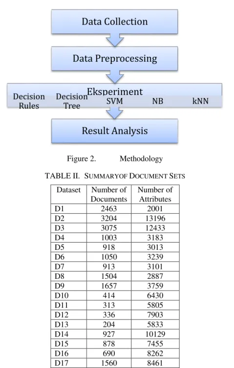
The steps that composes the methodology that is used in this research for comparing the performance of five text classification algorithms is shown in Fig 2.

This research was conducted in four main steps which are data collection, data preprocessing, experimentation, and result analysis. Collecting the text document needed for conducting the experiment is the first step in the methodology. The data is downloaded from http://weka.wikispaces.com/Datasets. These text documents then passed through preprocessing step. In preprocessing step documents are filtered and to transformed the data into ARFF format, the format accepted by WEKA. The first step in preprocessing is removing stop words such as number, prepositions (i.e. in, under, before), determiners (i.e. a, an another, the), and conjunctions (for, but, or, so, yet). The next step is grouping words that share the same morphological root, called stemming. The summary of dataset used is shown in Table II.

e-ISSN: 2477-8079 This article has been accepted for publication in Cogito Smart Figure 2. Methodology

TABLE II. SUMMARYOF DOCUMENT SETS

Dataset Number of Documents Number of Attributes D1 2463 2001 D2 3204 13196 D3 3075 12433 D4 1003 3183 D5 918 3013 D6 1050 3239 D7 913 3101 D8 1504 2887 D9 1657 3759 D10 414 6430 D11 313 5805 D12 336 7903 D13 204 5833 D14 927 10129 D15 878 7455 D16 690 8262 D17 1560 8461

The third step in the methodology is conducting the experiments. The datasets was tested using WEKA’s classifiers as shown in Table III.

TABLE III. WEKACLASSIFIERS

Algorithms Classifier

Decision Rule java weka.classifiers.rules.ConjunctiveRule Decision Tree java weka.classifiers.trees.J48

k-NN java weka.classifiers.lazy.lBk

Naïve Bayes java

weka.classifiers.bayes.NaiveBayesMultinomial

Result Analysis

Eksperiment

Decision

Rules

Decision

Tree

SVM

NB

kNN

Data Preprocessing

Data Collection

e-ISSN: 2477-8079 This article has been accepted for publication in Cogito Smart

Algorithms Classifier

SVM java weka.classifiers.functions.SMO

3. RESULT AND DISCUSSION

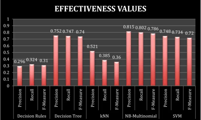
Algorithms comparison was done based on their accuracy, precision, recall, and F-Measure, and classifier model building time. As shown in Fig. 3 and Fig. 4, among the five algorithms, Naïve Bayes, Decision Tree, and SVM have high effectiveness and accuracy rates, Naïve Bayes classifier is the highest with 0.815, 0.802, and 0.786 respectively for Precision, Recall, and Measure. Directly proportional to the evaluation of precision, recall, and F-measure, Table III shows that naïve Bayes classifier has the highest accuracy rate among the five classifiers. The average accuracy of naïve Bayes is 80.33%. Decision Tree and SVM follow Naïve Bayes.

Figure 3. Average Classifer Effectiveness Values 0.296 0.324 0.31 0.752 0.747 0.74 0.521 0.385 0.36 0.815 0.802 0.786 0.748 0.734 0.72 0 0.1 0.2 0.3 0.4 0.5 0.6 0.7 0.8 0.9 1 Pr e cisio n R e ca ll F -M e a sure P re cisio n R e ca ll F -M e a sure Pr e cisio n R e ca ll F -M e a sure Pr e cisio n R e ca ll F -M e a sure Pr e cisio n R e ca ll F -M e a sure

Decision Rules Decision Tree kNN NB-Multinomial SVM

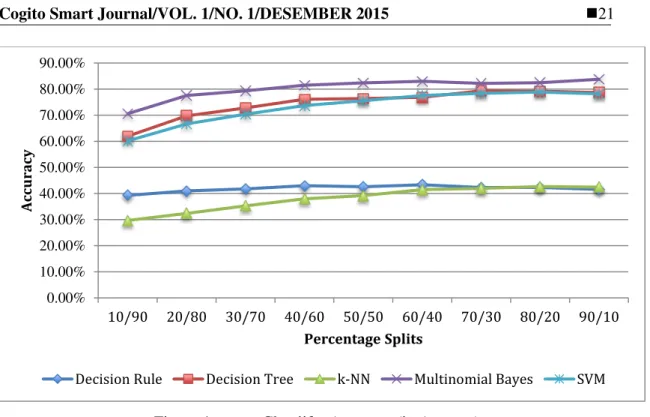
e-ISSN: 2477-8079 This article has been accepted for publication in Cogito Smart Figure 4. Classiifer Accuracy (in Average)

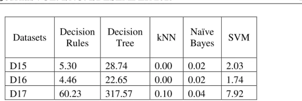
Another measure that is obtained from the experiment is the amount of time taken to build the classifier models (see Table IV). It shows that the average time required by k-NN classifiers is the smallest (fastest), 0.01 seconds. In contrast, decision tree classifiers take a long time to build a text classifier models. The average amount of time to accomplish building the model is 101.3 seconds.

TABLE IV. CLASSIFIER ACCURACY

Datasets Decision Rules Decision Tree kNN Naïve Bayes SVM D1 10.39 96.53 0.01 0.05 6.53 D2 36.85 570.86 0.01 0.07 13.15 D3 29.83 405.07 0.01 0.05 11.77 D4 1.31 20.46 0.00 0.01 1.24 D5 0.94 17.58 0.00 0.02 1.15 D6 1.25 26.56 0.00 0.01 1.53 D7 1.62 23.07 0.00 0.01 1.26 D8 7.83 42.92 0.01 0.01 2.86 D9 8.56 84.85 0.00 0.01 6.54 D10 1.84 11.81 0.00 0.01 0.73 D11 1.65 6.94 0.00 0.02 0.55 D12 1.25 12.52 0.00 0.03 0.87 D13 0.69 2.31 0.00 0.01 0.24 D14 0.00 31.65 0.00 0.02 2.21 0.00% 10.00% 20.00% 30.00% 40.00% 50.00% 60.00% 70.00% 80.00% 90.00% 10/90 20/80 30/70 40/60 50/50 60/40 70/30 80/20 90/10 Ac cu ra cy Percentage Splits

e-ISSN: 2477-8079 This article has been accepted for publication in Cogito Smart Datasets Decision Rules Decision Tree kNN Naïve Bayes SVM D15 5.30 28.74 0.00 0.02 2.03 D16 4.46 22.65 0.00 0.02 1.74 D17 60.23 317.57 0.10 0.04 7.92

In Table V we try to conclude the relation between classifier effectiveness values with amount of time taken to build classifier models. Both decision rules and k-NN have poor classification performance. Compare to k-NN, decision rules has the lowest in terms of precision and F-measure. Yet, its accuracy is higher than k-NN’s. SVM can reach high effectiveness performance (73.3%) in average of time 3.67 seconds for building a classification model. In terms of time, decision tree requires a huge amount of time to build classification model. However, it can classify the documents well. Overall, results of the experiment indicate that Naïve Bayes algorithm is superior among the five algorithms, assessed from the aspects of effectiveness and time. It requires small amount of time to build the model with high accuracy and effectiveness.

TABLE V. ACCURACY AND TIME TO BUILD THE MODEL

Algorithms Accuracy

(%) Precision Recall F-Measure

Time (second) Decision Rules 41.92 0.28 0.42 0.31 10.24 Decision Tree 74.59 0.75 0.75 0.74 101.3 k-NN 38.14 0.52 0.39 0.36 0.01 Naïve Bayes 80.33 0.82 0.8 0.79 0.02 SVM 73.3 0.75 0.73 0.72 3.67 4. CONCLUSION

This study compared performance of five machine learning based classification algorithms, namely decision rules, decision tree, k-NN, naïve Bayes, and SVM. Comparison was based on time and four classifier effectiveness measurements: precision, recall, F-measure, and accuracy. The following conclusions were drawn:

1. Decision rules and k-NN performance are lack since their effectiveness values and accuracy are less than

2. The algorithms that can build classifiers with high effectiveness rate are Naïve Bayes, decision tree, and SVM

a. SVM is able to classify the documents well in small amount of model building time. b. Decision tree have an equally good performance in classifying multi-class text

documents, with average precision, recall, and F-measure values more than 0.7, as well as accuracy rate which is around 75%. Yet, it has drawback in time to build the classifier models.

c. Experiment result shows Naïve Bayes has the highest effectiveness values, as well as spent small amount of time to build the classifier models.

3. Regarding the time taken to build classifier model, k-NN is the fastest, while decision tree is the slowest. Using the chosen datasets, k-NN can build a model in average of 0.01 second. Decision tree requires average of 101.3 seconds to build a model.

e-ISSN: 2477-8079 This article has been accepted for publication in Cogito Smart For Naïve Bayes and SVM algorithms, the greater the percentage of training documents, the higher the resulting model accuracy. Therefore, Naïve Bayes’ get the highest accuracy at percentage split of 90/10, while SVM is at 80/20 and decision tree is at 70/30.

REFERENCES

[1] H.Brucher, G. Knolmayer, and M.A. Mittermayer ., “Document Classification Methods for Organizing Explicit Knowledge”, Proceedings of the 3rd _{European Conference on} Organizational Knowledge, Learning, and Capabilities, Athens, Greece, 2002.

[2] F. Sebastiani, “Machine Learning in Autmated Text Categorization”, ACM Computing Surveys, Vol. 34, No. 1, pp. 1–47, March 2002,.

[3] S. Ramasundaram & S.P. Victor, “Algorithms for Text Categorization: A Comparative Study”, World Applied Sciences Journal, Vol. 22, No.9, pp. 1232-1240, 2013.

[4] E. Leopold & J. Kindermann, “Text Categorization with Support Vector Machines. How to Represent Texts in Input space?”, Machine Learning 46, pp. 423-444, 2002.

[5] M. Ikonomakis, S. Kotsiantis, & V. Tampakas, “Text Classification Using Machine Learning Techniques”, WEAS Transactions on Computers, Vol. 4, No. 8, pp. 966-975, August 2005.

[6] C. Goller, et.al., Automatic Document Classification: A Thorough Evaluation of Various Methods, Proceedings of Internationalen Symposiums Informationsgesellschaft, 2000. [7] C. C. Aggarwal & C. X. Zhai, “A Survey of Text Classification Algorithms”, in Mining

Text Data, Springer Science Business Media, 2012.

[8] A. Bratko & B. Filipié, A Study of Approaches to Semi-structured Document Classification, Technical Report IJS-DP 9015, Josef Stefan Institute, Slovenia, 2004. [9] Y. Yang. & X. Liu, “A Re-examination of Text Categorization Methods”, Proceedings of

SIGIR-99, 22nd _{ACM International Conference on Research and Development in} Information Retrieval, New York, US, pp.42-49 1999,

[10] J.Han & M. Kamber, Data Mining Concepts and Techniques, Academic Press,USA, 2001.

[11] I. H. Witten & Eibe Frank, Data Mining Practical Machine Learning Tools and Techniques, Edisi Kedua, Morgan Kaufmann Publishers, 2005.