A multiple-point spatially weighted k-NN classifier for remote sensing

A multiple-point spatially weighted k-NN classifier for remote sensing

Yunwei Tang

, Linhai Jing

, Peter M. Atkinson

, and Hui Li

a

Key Laboratory of Digital Earth Science, Institute of Remote Sensing and Digital Earth, Chinese Academy of Sciences, Beijing, China; bFaculty of Science and Technology, Engineering Building, Lancaster University, Lancaster, UK; cSchool of Geography, Archaeology and Palaeoecology, Queen’s University Belfast, Northern Ireland, UK; dGeography and Environment, University of Southampton, Southampton, UK

Yunwei Tanga, Linhai Jinga, Peter M. Atkinsonb, c, d, Hui Lia

a

Key Laboratory of Digital Earth Sciences, Institute of Remote Sensing and Digital Earth, Chinese Academy of Sciences, No. 9 Dengzhuang South Road, Beijing 100094, China

b

Faculty of Science and Technology, Engineering Building, Lancaster University, Lancaster LA1 4YR, UK

c

School of Geography, Archaeology and Palaeoecology, Queen’s University Belfast, Belfast BT7 1NN, Northern Ireland, UK

d

Geography and Environment, University of Southampton, Highfield, Southampton SO17 1BJ, UK

Corresponding author: Yunwei Tang Email: [email protected] Linhai Jing Email: [email protected]

The paper was supported by the [National Science and Technology Support Program] under Grant [2013DFG21640]; the [National Natural Science Foundation of China] under Grant [41501489]; the [100 Talents Program of the Chinese Academy of Science]

under Grant [Y34005101A]; and the [Major Program of High Resolution Earth Observation System] under Grant [30-Y20A37-9003-15/17].

A multiple-point spatially weighted k-NN classifier for remote sensing

proposed in this paper. The method is a modified version of the spatially weighted k-nearest neighbour (k-NN) classifier, which accounts for spatial correlation through weights applied to neighbouring pixels. The MPS

characterises the spatial correlation between multiple points of land cover classes by learning local patterns in a training image. This rich spatial information is then converted to multiple-point probabilities and incorporated into the k-NN

classifier. Experiments were conducted in two study areas, in which the proposed method for classification was tested on a WorldView-2 subscene of the Sichuan mountainous area and an IKONOS image of the Beijing urban area. The multiple-point weighted k-NN method (MPk-NN) was compared to several alternatives; including the traditional k-NN and two previously published spatially weighted k-NN schemes; the inverse distance weighted k-NN, and the geostatistically weighted k-NN. The classifiers using the Bayesian and support vector machine (SVM) methods, and these classifiers weighted with spatial context using the Markov random field (MRF) model, were also introduced to provide a benchmark comparison with the MPk-NN method. The proposed approach increased classification accuracy significantly relative to the alternatives, and it is, thus, recommended for the identification of land cover types with complex and diverse spatial distributions.

Keywords: multiple-point statistics; k-NN; classification; training image

1. Introduction

The use of remotely sensed data for the classification of land cover is important for a wide range of applications. Numerous methods have been proposed for increasing the accuracy of classification. Amongst these, contextual classifiers, which use spatial information along with spectral information, can potentially achieve greater accuracy than non-contextual classifiers (Magnussen, Boudewyn, and Wulder 2004; Ghimire, Rogan, and Miller 2010; Pasolli et al. 2014). The spatial contextual classifier known as the Markov random field (MRF) method is popular and has been shown to increase

classification accuracy (Solberg, Taxt, and Jain 1996; Sun et al. 2016). Geostatistics is a useful framework for modelling spatial data and quantifying spatial dependence, and it has shown some promise for contextual classification (Atkinson and Lewis 2000). However, the spatial weighting established using geostatistics is based on two-point statistics, failing to describe the joint variability at three or more points at a time (Strebelle 2002).

Multiple-point statistics (MPS) has been proposed as a development of traditional geostatistics (Guardiano and Srivastava 1993). Instead of two-point-based functions such as the variogram, MPS borrows rich spatial structure information from training images, from which the local patterns of the target field can be constructed. Recently, a few studies applied MPS to the classification of remote sensing data. For example, Ge and Bai (2011) extracted linear objects from remotely sensed imagery using MPS. Tang et al. (2013) proposed a post-classification method based on MPS and compared it with contextual classification methods. Ge (2013) explored a sub-pixel mapping method, in which the MPS method was applied to characterise the spatial structural properties of surface objects. However, most studies related to classification using MPS increased the accuracy by simply combining the spatial and spectral information or applying the MPS directly to the classification result rather than improving the classifier itself.

The k-nearest neighbour (k-NN) classifier retains the location information associated with training data, such that a geographical weighting can be integrated readily into the classifier. It has been shown that both a distance weighting scheme and a geostatistical (variogram) scheme can lead to sound classification results (Atkinson and Naser 2010). It is, therefore, of interest to explore whether replacing the variogram with MPS can further increase the achievable accuracy. The objective of this paper was,

thus, to introduce the MPS-based spatial weighting into the k-NN classifier in order to extract the spatial structure of the multiple class distribution, then the spatial

information can be converted to the multiple-point probability combined with the spectral information to increase the accuracy of the k-NN classifier. A WorldView-2 image in the Sichuan mountainous region and an IKONOS image in the Beijing urban area of China were used to assess the new method in comparison to classifiers based on spectral information and other types of spatial weighting.

2. Methods

The training image, data event, and multi-grid concepts in MPS are applied here to the proposed MPS-based classification method, so these concepts are introduced briefly in this section. Then the multiple-point weighted k-NN method is presented, with a brief review of the traditional distance-weighted and the alternative geostatistically-weighted

k-NN methods.

2.1. The MPS approach

MPS characterises spatial dependence from a training image, which should be chosen to depict the types of structures that the area of interest exhibits. A training image

substitutes for the variogram or covariance function in traditional geostatistics, and provides the prior knowledge required for spatial correlation modelling. A data template, composed of multiple nodes with any user-specified configuration, is used to scan the training image, and the number of replicates of each different data event is retrieved (Liu, 2006). A data template with a central node u is defined as T(u) = {h1, …, hn},

which is composed of n locations ui (i = 1, …, n), where hi is a vector (for both distance

and direction) between ui and u. The data template T(u) is used to scan the training

categorical values and is obtained by the (geometrically) same template that is used to scan the training image. A data event can be expressed as dev(u) = {c(u1), …, c(un)},

where c(ui) (i = 1, …, n) is the categorical value at location ui within the template

(Okabe and Blunt 2005).

The number of replicates of a data event can be calculated when the training image is scanned by the template, and the relative frequency of each data event can be converted to a conditional probability. Only those proportions corresponding to the data events actually found over the training image are utilised directly as conditional

probabilities without any prior modelling (Strebelle 2002).

The multi-grid simulation approach can be adopted in MPS to capture structures of different sizes in the training image (Tran 1994). The multi-grid approach expands the size of the simulated grid while not increasing the number of nodes. It is assumed that the data template T(u) has L multi-grid levels. The new geometrical template is constructed by rescaling the original template such that TL( )u 





2.2. Multiple-point weighted k-NN

In the traditional k-NN method, the classifier allocates pixels to the neighbours to which it is closest in feature space. An inverse distance weighting (IDW) function can be incorporated into the k-NN classifier to give more weight to information from a neighbour close to an unclassified observation than from a more distant neighbour (Dudani 1976). IDW can be expressed as:

, , 1 u k p u k d   (1)

where du,k measures the distance between the current pixel u and its neighbouring

exponent p is an integer that determines the magnitude of the weight. The term wk-NN is used to refer to the IDW-based k-NN method.

In a geostatistically weighted k-NN classifier (gk-NN), the probability that a pixel u belongs to class m can be evaluated as follows (Atkinson and Naser 2010):

 





 









 













where the subscript u,k of h indicates the distance and direction between pixel u and its neighbour k.

p

 

h

m is the class of interest. Sg is a proportional weight between 0 and 1.

In the proposed MPS-based k-NN approach, instead of training samples, the conditional probability is derived from the training image to provide spatial information. For an unknown location u (i.e., the category of u needs to be estimated), k nearest neighbour training pixels uk can be found. Thus, the data template at location u can be

defined as T(u) = {h1, …, hk}, where hk is measures the distance and direction between

uk and u. So the template centred at u consists of the same separation vector hk and the

same classes with the neighbouring k pixels. This template is used to scan the training image and derive the multiple-point probability for pixel u by counting the replicates of the data event dev(u), where dev(u) = {c(u1), …, c(uk)}. The probability of pixel u with

class m equals the proportion of the number of dev(u) that possesses class m at the central node to the total number of dev(u). For another pixel, a different template is

applied to estimate another probability from the training image. The multiple-point probability that a pixel u belongs to class m is, thus, expressed as:

 







 

 



 









Note that dev(u) = 1 means that the data event dev(u) is found in the training image, indicating that all k pixels at location uk should match exactly the corresponding

classes (i.e., c(uk) = mk). The indicator function I takes a value of one if the condition is

satisfied, otherwise zero. Thus, the multiple-point based k-NN classifier (MPk-NN in brief) can be written as:

 





 











 



 

 





 











 







 

















Similar to Sg, SMP is a multiple-point statistical weight given to the classifier,

ranging from 0 to 1.

To estimate the multiple-point probability in the MPk-NN method, a training image is defined. It can be obtained either for the same area that needs to be classified using the MPk-NN method or represent a different place. However, the training image is required to have a similar class spatial distribution to that of the study area and, thus, to provide prior knowledge on the character of spatial information. The data template is

then defined, which consists of k nearest neighbour pixels of the current pixel.

Therefore, one pixel in the image corresponds to only one data template, and the data templates are different at each location. The multi-grid concept is applied to the data template. Instead of expanding the data template, the rescaled template is constructed by condensing the original one. Thus, the data template is formed as:





1

( ) 2 , , 2

L L L

n

T u  h  h  . Figure 1 displays an example of data template

construction, the process of estimating the multiple-point probability, and the data templates with a multi-grid level L of 3.

[Figure 1 near here]

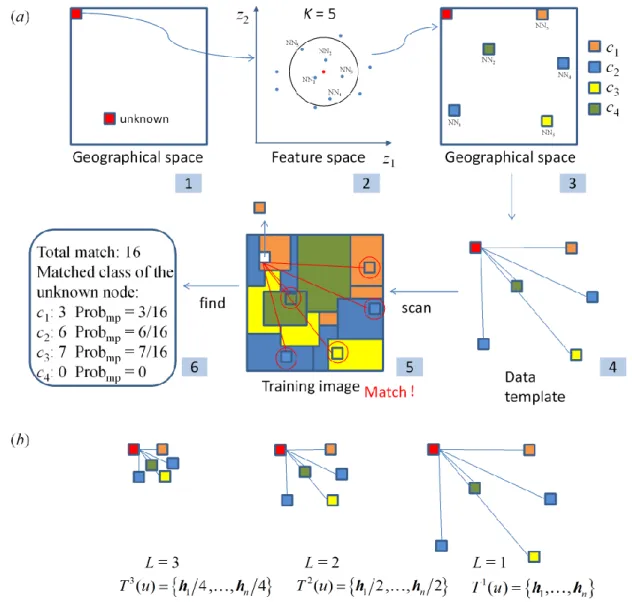
As shown in Figure 1(a), to estimate the category of a pixel in an image (geographical space) (step 1), the k-NN method first projects this pixel into feature space, which is usually constructed with the spectral dimensions of the image. Then k

nearest neighbouring training pixels in feature space related to the unknown pixel are found, for example, k = 5 (step 2). Among 5 training pixels, if 3 pixels belong to categories 1, 3, and 4, respectively, and 2 pixels belong to category 2, then this pixel is classified as category 2 using the k-NN classifier, determined by majority voting. 5-NN training pixels are then projected back to geographical space (step 3). The data template is constructed by the 5-NN training pixels centred on the unknown pixel (although the unknown pixel may not be the centre in geographical space). This data template corresponds only to the current unknown pixel, and this is used to scan the training image (step 4). In the scanning process, the categories of all the 5 pixels in the data template should be exactly matched (i.e., a data event is matched), then the current category at the centre of the data template is recorded, for example, category 1 (step 5). The scanning process is from top to bottom and left to right of the training image. For simplicity, we assume that 16 matched data events are found by this data template after

scanning the whole training image. And among 16 data events, 3 nodes at the centre of the data template belong to category 1, 6 nodes belong to category 2, 7 nodes belong to category 3, and none belong to category 4. Thus, the multiple-point probabilities are 3/16, 6/16, 7/16 and 0 for the four categories (step 6). Figure 1(b) shows the compact multi-grid data templates. For example, if L is taken as 3, the data template was 1/2 and 1/4 of the original one for L = 2 and 3, respectively.

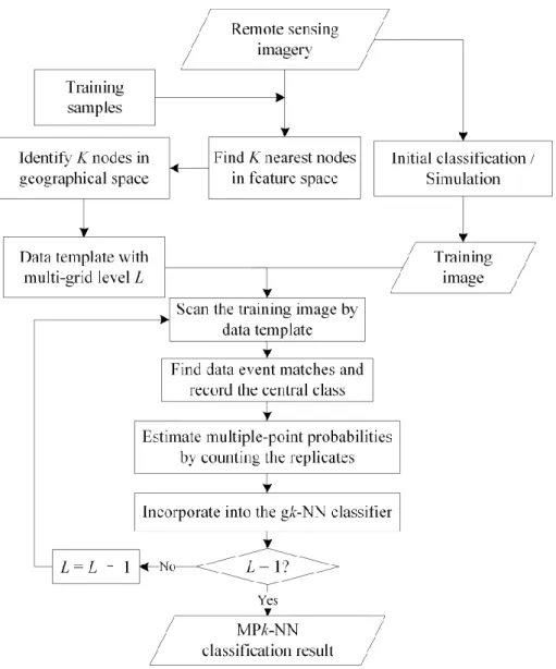
A flowchart representing the MPk-NN classification process is shown in Figure 2. A remotely sensed image and training samples for classification are first provided, along with a training image, which reflects the desired spatial pattern and provides prior information on the area of interest. Here, for a fair comparison with other classification methods, the training image is derived from an initial classification or a simulation result. Then the data template is constructed using the k-NN rule as shown in Figure 1(a), and the multi-grid data templates at each location are used to scan the training image. The replicates of the data events are recorded according to the class type of the central node (the red node in Figure 1(a)). This information is then converted to a conditional probability for each class and incorporated into the gk-NN classifier, as shown in Equation (4).

[Figure 2 near here]

3. Case study

3.1. Study area and data processing

The wild giant panda (Ailuropoda melanoleuca) lives in a few mountain ranges in central China, mainly in Sichuan Province, where bamboos act as the main food source. Estimating and mapping suitable habitat plays a critical role in conservation planning and the development of policy for endangered species. Therefore, knowledge of the

spatial distribution of bamboos is important for identifying suitable habitat for giant pandas.

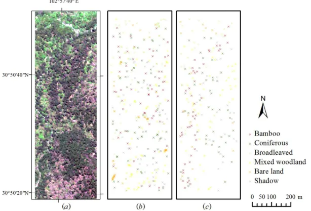
The first study site is located at Dengsheng Ditch in Wolong region, Sichuan Province, China. The study area is shown in Figure 3(a). The image is a subscene (30°50ʹ19ʺ–30°50ʹ51ʺN, 102°57ʹ35ʺ–102°57ʹ48ʺE) from WorldView-2 imagery with size 493  161 pixels, acquired on 28 May 2014. The dataset consists of eight

multispectral bands with a spatial resolution of 2 m. The altitude of Dengsheng Ditch is from 2.7 to 4.5 km. The area is covered by various species of vegetation, the forest cover types of which are defined as bamboo, coniferous, broadleaved, and mixed woodland. Two further categories were included in the classification: bare land and shadow.

Extensive fieldwork at Dengsheng Ditch was carried out in two field visits. The first was on 13 June 2014, with the aim of measuring feature points for image geometric correction and the collection of training samples. The second field visit occurred on 12 September 2014, for the purpose of testing the accuracy of the classification. A

Trimble○R GeoXHTM 6000 handheld GPS was used to collect location points. An antenna was connected to the GPS to ensure that the signal could be received from more than three satellites under the canopy of large trees.

[Figure 3 near here]

When collecting sample points in the field, only four types of forest cover (bamboo, coniferous, broadleaved, and mixed woodland) were recorded. The sample points of bare land and shadow were chosen manually from the image, since they were easy identifiable and thus no ground control points were collected. Of 576 sample points, 365 sample points were used for training and 211 points were used for testing. The numbers of training samples are 57, 68, 63, 63, 51 and 63 for the classes of bamboo,

coniferous, broadleaved, mixed woodland, bare land and shadow, respectively. The spatial distributions of the sample points are shown in Figure 3(b) and 3(c). The sample points of the bamboo class account for a larger proportion because they were

specifically targeted in the fieldwork, although coniferous and mixed woodland are the main forest covers in the area.

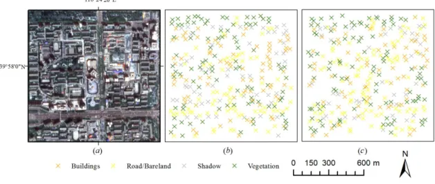
Another case study was undertaken on an IKONOS image (39°57ʹ55ʺ–

39°58ʹ28ʺN, 116°24ʹ5ʺ–116°24ʹ49ʺE) with size 256  256 pixels over the Beijing urban area (Figure 4(a)), acquired in May 2000. The IKONOS dataset consists of four

multispectral bands with a spatial resolution of 4 m. The typical urban area can be classified generally into four high-level classes: buildings, vegetation, road/bare land and shadow. Since the four classes in the IKONOS image can be identified readily by visual inspection, the training and testing samples were labelled manually in the image. 600 points in total were selected as samples, among which, 300 points were used for training and 300 points were used for testing. The numbers of training samples are 80, 94, 72 and 54 for the classes of buildings, vegetation, road/bare land and shadow, respectively. The spatial distributions of the sample points are shown in Figure 4(b) and 4(c).

[Figure 4 near here]

3.2. Classification

The classification process was the same for both study areas. To provide benchmarks, the traditional k-NN classifier was first applied to all the multispectral bands based on the spectral values of each pixel, with a value of k equal to 5. wk-NN classification was then performed given the same training samples. The IDW scheme was used in the k

-NN classifier with an exponent parameter p of 2 in Equation (1). gk-NN is a two-point statistical weighted method. The class-conditional probability plots were estimated from the same training points used for classification, and then fitted with covariance-type models.

To compare the proposed method with other state-of-the-art classifiers, two popular classification methods were applied: the Bayesian and support vector machine (SVM) methods. Also, previous studies have shown the advantages using the MRF spatial contextual classifier to improve both the Bayesian and SVM classification methods (Wu and Ouyang 2011; Moser and Serpico 2013). Therefore, the spatial weighting using MRF was also applied to the Bayesian and SVM methods to provide a further benchmark comparison with the MPS-based weighting method. The radial basis function (RBF) kernel function was used in the SVM method. A 10-fold

cross-validation was applied to select optimal parameters (the penalisation constant C and the kernel parameter γ) for RBF kernel. It is found that the optimal parameter C = 1 and γ = 0.0125 with the mean accuracy equals 96.5% and the standard deviation equals 0.076 for the Wolong case study, and C = 0.8 and γ = 0.0053 with the mean accuracy equals 98.7% and the standard deviation equals 0.018 for the Beijing case study. The simulated annealing optimisation approach using a Gibbs sampler was employed in the MRF model (Berthod et al. 1996).

Here, the training image was produced using the spatially smoothed gk-NN classification result. The data template for each pixel consisted of five nearest neighbour nodes. The multi-grid level L was taken as 3, and the multiple-point statistical weight

SMP was set as 0.6 for the Wolong case study and 0.8 for the Beijing case study, which

3.3. Results

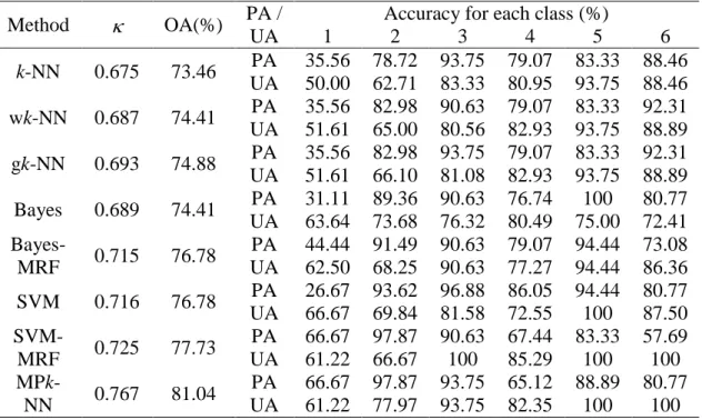
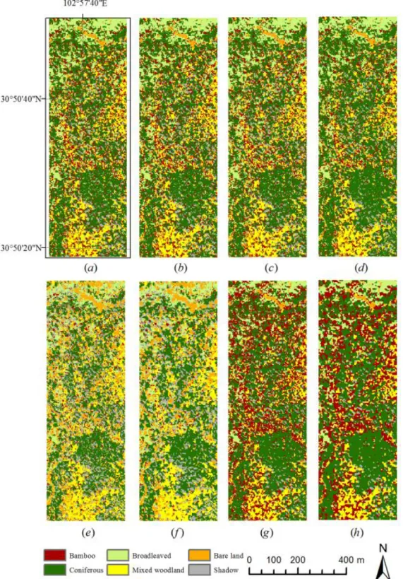
In the Wolong case study, the classification results obtained using the proposed method and the seven benchmark methods are displayed in Figure 5, and the classification accuracies are summarised in Table 1. As can be seen, in terms of overall accuracy, the proposed MPk-NN method produced an accuracy of 81.04% compared to the traditional

k-NN method for which the accuracy was only 73.46%. The two spatial k-NN methods produced accuracies of 74.41% (wk-NN) and 74.88% (gk-NN), which lie somewhere between the non-spatial k-NN method and the proposed method. The overall accuracies are 74.41% and 76.78% using the Bayesian and SVM methods, which are greater than the traditional k-NN methods. Then the MRF model further increased the accuracies to 76.78% and 77.73% using the Bayesian and SVM classifiers, respectively. Nevertheless, the overall accuracy and the kappa coefficient () of the MPk-NN result are the largest, which indicates the MPS spatial weighting increases the accuracy of classification more than the MRF weighting.

[Figure 5 near here] [Table 1 near here]

The four k-NN results in Figures 5(a)-(d) are very similar. The bamboo class appears more commonly in the k-NN result, but with the lowest user’s accuracy. This is because the k-NN method is sensitive to sample size, and the number of training

samples for the bamboo class is the largest among all the classes. The gk-NN method has a greater overall accuracy and  than the wk-NN method. In fact, a large distributed class patch in the wk-NN result was not modified using the gk-NN method; in most cases, the gk-NN changed the allocation of mixed pixels near the land cover borders. In the MPk-NN result in Figure 5(d), the area of coniferous woodland in the lower right of

the image is spatially smoother than the same area in the other classification results, which indicates that MPk-NN can act as an effective smoother to increase classification accuracy. Two of the Bayesian results have the least pixels allocated to the bamboo class, whereas the number of pixels in the bamboo class in two of the SVM results is the largest. However, the producer’s accuracies of the bamboo class are both very low for the Bayesian and SVM methods. The MRF-based methods in Figure 5(f) and (h) spatially smoothed the classification results according to the neighbouring classes compared to the original results in Figure 5(e) and (g), leading to an increase in the producer’s accuracies of the bamboo class. In fact, bamboos are covered by tree crowns at most locations in the study area. Therefore, bamboos are usually sparsely distributed as fragments only, and many pixels were misclassified as bamboos in the centre of the image.

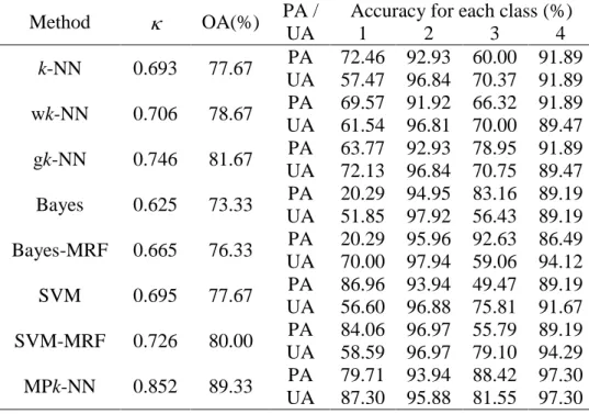
Since the environment is complex in Wolong, and the forest covers are not very easily be identified, the second case study in the urban area of Beijing was introduced. The classification results are displayed in Figure 6, and the classification accuracies are summarised in Table 2. As shown in Table 2, similarly, the two weighted k-NN

methods produced greater overall accuracies (78.67% for wk-NN and 81.67% for gk -NN) than the traditional k-NN method (77.67%), whereas the MPk-NN has the greatest overall accuracy (89.33%) and . Different from the previous case study, the Bayesian (73.33%) and SVM (77.67%) methods do not show an advantage over the k-NN classifier, but the MRF weighting still increased the accuracies compared to the non-spatial methods (76.33% for Bayesian with MRF and 80.00% for SVM with MRF).

[Figure 6 near here] [Table 2 near here]

In this case, it is difficult to distinguish buildings from road/bare land since these two classes have similar spectral responses. Many pixels belonging to the building class were obviously misclassified as road/bare land in the Bayesian result in Figure 6(e), and the MRF-based result in Figure 6(f) further smoothed the building class, leading to the greatest producer’s accuracy of the road/bare land class. In the SVM result in Figure 6(g), on the other hand, some roads in the upper right and some bare land classes in the centre of the image were misclassified as buildings. Through MRF smoothing, some pixels were corrected in the upper right of the image, but some bare land classes in the centre were still allocated as buildings in Figure 6(h). The k-NN result in Figure 6(a) distinguished these two classes, although the classified map appears more noisy than the Bayesian and SVM results. The wk-NN result in Figure 6(b) does not show much difference from the traditional k-NN result in Figure 6(a), whereas the gk-NN result in Figure 6(c) changed some pixels from buildings to the road/bare land class, improving the producer’s accuracy of the road/bare land class. The MPk-NN result in Figure 6(d) clearly shows a smoothing effect. But unlike the MRF weighting, which filters the noise and smooths the edges according to neighbouring information, the MPS-based

weighting accounts for the dominant spatial patterns in the training image. When applying a post-processor such as a mean filter to smooth an image, the processor is operating on the result of the classification. Here, the MPk-NN is a more sophisticated form of post-processing where the processor borrows structures from other parts of the training image, and at varying spatial resolutions using multi-grid data templates, in order to update the gk-NN classified image.

3.4. Significance test and higher-order statistics

An analysis of variance (ANOVA) for the classification accuracy was performed using the F-test. To do so, the classification results were first compared to testing data. A

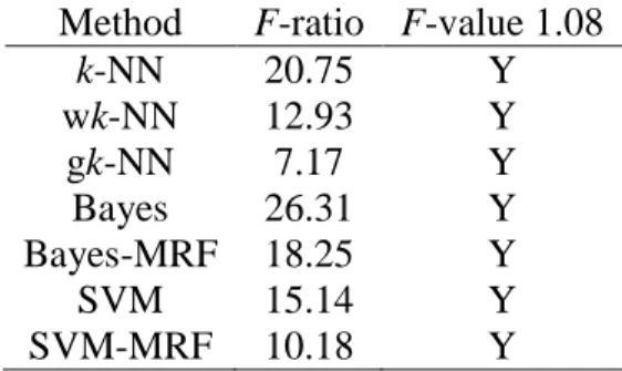
binary variable was created for each method representing classification success/failure (the variable was set to one if the classification value equals the testing data, otherwise zero). Then all the results were compared with the MPk-NN result. As shown in Tables 3 and 4, the MPk-NN result produced significant increases in accuracy with respect to all the classification results at the 70% confidence interval except for the SVM

classification weighted with the MRF model in the Wolong case study. It indicates that it is worth applying the MPS-based weighting to increase the classification accuracy compared to the other classification methods and spatial weightings. In fact, in the case study of Beijing, the increase in accuracy of the MPk-NN method reached 90%

confidence level compared to all the other methods, in which the F-value equals 2.71. Therefore, although Tables 1 and 2 show that the MPk-NN method does not always result in the greatest producer’s and user’s accuracy for each class, it has a greater probability to provide a significant increase in overall accuracy than the other methods.

[Table 3 near here] [Table 4 near here]

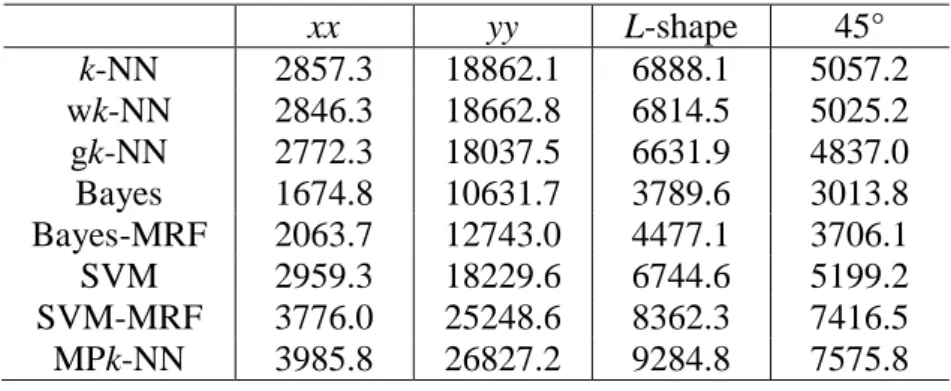
We applied higher-order statistics to the classification results to investigate the ability of the classifiers to recreate the desired spatial patterns. A three-node template was used to detect the correlation between the start point and two other points away from the start point at distances h1 and h2 along the given direction (Dimitrakopoulos,

Mustapha, and Gloaguen 2010). Four templates were used: templates with two distances both along the x axis and both along the y axis, an L-shaped template with two distances along the x and y axes, and a template with two distances both along 45°

counter-clockwise from the x axis. A third-order cumulant statistic for each class was estimated. The class in focus was set as one and other classes were set as zero. Thus, the classes of

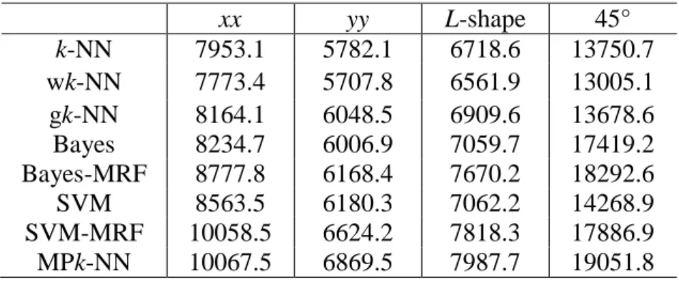
all the three nodes in the template are required to be the same to result in one for the third-order cumulant statistic. Tables 5 and 6 show the summation of the cumulants for all the classes, which reflects the overall connectivity of the spatial patterns and the spatial correlation within classes for the classification results. It can be seen that the MPk-NN always yields the largest cumulant, contributed by the statistics captured from multiple points. The results indicate that the predicted spatial patterns for MPk-NN generally have greater connectivity and spatial correlation than the other methods.

[Table 5 near here] [Table 6 near here]

4. Discussion

4.1. Parameter analysis

Several parameters were introduced to the MPk-NN method in Equation (4), which are worth further discussion. Firstly, the number of NN pixels k is considered. Much research has discussed the choice of k in the k-NN classifier (Ghosh 2006; Hassanat et al. 2014). What is different here from the traditional k-NN method is that the data templates used in the MPS are also constrained by the number of k. Thus, if k is set to a very large value, the classification takes a longer time, and it is possible that no data event can be found in the training image by the strict conditioning of the data template. If the data template cannot find any matched data event, then the multiple-point

probability of the corresponding pixel equals 0, which means that the MPS does not provide any weighting information to this pixel. Here, we set k as 5 in the experiments. The percentages of the pixels that failed to produce a multiple-point probability under the three multi-grid levels were 4.7% and 3.4% for the two case studies, respectively. Therefore, it is not suggested to take a value larger than 5 in the MPk-NN method.

Conversely, a smaller value k may decrease the classification accuracy as a result of choosing the majority class in feature space from a smaller number k of neighbours. The multi-grid template in the MPk-NN method is derived from the nearest neighbour nodes, which is different to the locally compact window commonly used in MPS. It may be preferable to restrict the template to be more compact because the template can sometimes be spatially extensive, and expanding the template may fail to capture data events inside a spatially limited training image. Also, a spatially limited template may be more suited to capturing spatial dependence since near things tend to be similar. Taking the value 3 for the number of multi-grid levels is a common choice in the MPS, and a larger value would increase the scanning time. However, sometimes the template is already small at the original scale, in which case it is not necessary to further condense the template. Future research should, therefore, be focused on the use of appropriate multi-grid levels for different templates. For example, small data templates are only used at the original grid level, whereas large data templates are used at smaller grid levels to ensure that at least one data event can be matched until the template cannot be condensed.

Since the multiple-point weight SMP was introduced in the MPk-NN method, a

sensitivity analysis was performed. The sensitivity analysis was undertaken for the case study of Beijing only. The overall accuracy, and the user’s and producer’s accuracies of the classes of buildings and road/bare land were tested against a varying weight SMP

from 0.1 to 0.9. The result is shown in Figure 7. As can be seen, the overall accuracy is larger than for the other k-NN methods when SMP varies from 0.3 to 0.9. SMP was taken

as 0.8 because it resulted in the greatest overall accuracy. It is of interest to compare the spatial information of MPS with the spatial covariance provided by traditional

distance. Thus, it may have a large effect via the spatial weighting, even if the data template is large. Secondly, the spatial covariance measures the spatial correlation between the central node and one of its k-NN nodes at one time; MPS summarises the correlation of the central node and all of its k-NN nodes. Finally, because of the second difference, the weight factor SMP accounts for more weight than Sg. Thus, it may not

take a large value. For example, SMP was set to 0.6 in the case study of Wolong.

[Figure 7 near here]

4.2. Training image test

It should be noted that the training image introduced in the MPk-NN method is

generally not available in the other methods. However, to demonstrate the power of the proposed method, and to avoid using new data and, thus, provide a fair comparison with the benchmarks, the training image used in the present implementation of the MPk-NN method was a prior classification of the identical target area produced using the

common input dataset. In this implementation, the MPk-NN method acts in the same way as the other spatial k-NN classifiers, but reprocesses the rich multiple point spatial information in a previous classification map to determine the spatial weights.

Importantly, the MPk-NN classifier uses the previous classified map only as rich spatial structure information. It does not use the classified map as a starting point for further updating. Thus, the MPk-NN classifier effectively borrows spatial structure from multiple parts of the training image (class map) to condition the classification of other parts of the raw input image for which there may be uncertainty about the appropriate spatial structure. There are also important effects in terms of borrowing spatial

information across scales (e.g., using large spatial patterns found in the training image to condition the mapping of smaller patterns that are less well resolved).

When implemented in the above way the proposed method represents an increase in classification accuracy without the need for new data. In practice, however, generally the investigator may seek a training image from a different source and use that additional spatial information to condition the classification result. Here, a training image test was applied for the Beijing case study. Specifically, we tested the effects on the MPk-NN result of using different training images. As shown in Figure 8(a), the original training image was derived from the spatially smoothed gk-NN result. Four different training images were tested: a flipped training image of Figure 8(a) (not shown in Figure 8), a subset of the original training image (Figure 8(b)), a training image from a different area (Figure 8(c)), and a training image with the simplest pattern that

accounts only for the proportion of the four classes (Figure 8(d)). Under the same conditioning, the classification accuracies using the MPk-NN method with these four training images are (a) 83.33% (flipped image), (b) 85.33%, (c) 84.67% and (d) 81.67%. For the last training image with the simplest pattern, the resulting accuracy using the MPk-NN equals the accuracy using the gk-NN method (81.67%), which means this training image does not provide any useful information. The other training images increased the accuracy to a greater or lesser degree compared with the gk-NN method. However, the increase in accuracy was greatest for the original training image, since the original training image is of the same area. Therefore, the most important attribute of a training image is that it can reflect the desired spatial distribution of the target area. Which method is used to produce the training image and the per-point accuracy of the training image are of little concern. It is suggested to use a previous classification result or its derivatives as a training image to achieve a high classification accuracy. Moreover, in the present demonstration of the new MPk-NN method in this paper, this approach

has the added advantage that the new method does not use or require any new information relative to the benchmarks. Questions, however, still remain about the appropriateness and accuracy of the training image that may be selected, and this is currently the focus of much research in the field of MPS. Thus, future research should be focused on the selection of the training image and its effect to the MPS result.

5. Conclusion

This paper explored the potential of MPS for spatial weighting a remote sensing

classification. A new multiple-point statistical k-NN classification method was proposed and tested on two remotely sensed images. The new MPk-NN classification method can account for the multiple point spatial correlation provided by a training image, in contrast to common spatial weighting schemes, which are limited to two-point statistics or average neighbourhood information. The MPS-based weighting was compared to the IDW, geostatistical, and MRF contextual weighting schemes, and the MPk-NN method was compared to the Bayesian and SVM classifiers. The results demonstrated that greater classification accuracy can be achieved using the MPk-NN method. Although the proposed method was tested on the fine spatial resolution images, generalisations of the MPk-NN method for both at different spatial resolutions (e.g., Landsat dataset) and upon object-oriented method on fine spatial resolution images are expected to explore in the future.

Acknowledgements

The paper was supported by the [National Science and Technology Support Program] under Grant [2013DFG21640]; the [National Natural Science Foundation of China] under Grant [41501489]; the [100 Talents Program of the Chinese Academy of Science] under Grant [Y34005101A]; and the [Major Program of High Resolution Earth

Observation System] under Grant [30-Y20A37-9003-15/17]. The authors thank the Editor Prof. Arthur Cracknell and three anonymous reviewers for providing helpful suggestions that greatly improved the manuscript.

References

Atkinson, P. M., and P. Lewis. 2000. “Geostatistical Classification for Remote Sensing: An Introduction.” Computers & Geosciences 26: 361-371. doi:10.1016/S0098-3004(99)00117-X.

Atkinson, P. M., and D. K. Naser. 2010. “A Geostatistically Weighted K-NN Classifier for Remotely Sensed Imagery.” Geographical Analysis 42(2): 204-225. doi: 10.1111/j.1538-4632.2010.00790.x.

Dimitrakopoulos, R., H. Mustapha, and E. Gloaguen. 2010. “High-Order Statistics of Spatial Random Fields: Exploring Spatial Cumulants for Modeling Complex Non-Gaussian and Non-Linear Phenomena.” Mathematical Geosciences 42(1): 65-99. doi: 10.1007/s11004-009-9258-9.

Berthed, M., Z. Kato, S. Yu, and J. Zerubia. 1996. “Bayesian image classification using Markov random fields.” Image and Vision Computing 14(4): 285-295. doi:10.1016/0262-8856(95)01072-6.

Dudani, S. A. 1976. “The Distance Weighted K-Nearest Neighbour Rule.” IEEE Transactions on Systems Man, and Cybernetics SMC-6(4): 325-327. doi:10.1109/TSMC.1976.5408784.

Ge, Y., and H. Bai. 2011. “Multiple-Point Simulation-Based Method for Extraction of Objects with Spatial Structure from Remotely Sensed Imagery.” International Journal of Remote Sensing 32(8): 2311-2335.doi:10.1080/01431161003698278. Ge, Y. 2013. “Sub-Pixel Land-Cover Mapping with Improved Fraction Images upon

Multiple-Point Simulation.” International Journal of Applied Earth Observation and Geoinformation 22: 115-126. doi:10.1016/j.jag.2012.04.013.

Ghimire, B., J. Rogan., and J. Miller. 2010. “Contextual Land-Cover Classification: Incorporating Spatial Dependence in Land-Cover Classification Models Using Random Forests and the Getis Statistic.” Remote Sensing Letters 1(1): 45-54. doi:10.1080/01431160903252327.

Ghosh, A. K. 2006. “On Optimum Choice of K in Nearest Neighbor Classification.”

Computational Statistics & Data Analysis 50(11): 3113-3123. doi: doi:10.1016/j.csda.2005.06.007.

Guardiano, F., and R. M. Srivastava. 1993. “Multivariate geostatistics: beyond bivariate moments.” In Geostatistics Tróia’92, edited by Amilcar Soares, 133-144. Dordrecht: Kluwer Academic Publications.

Hassanat, A. B., M. A. Abbadi, G. A. Altarawneh, and A. A. Alhasanat. 2014. “Solving the Problem of the K Paramter in the KNN Classifier Using an Ensemble Learning Approach.” International Journal of Computer Science and Information Security

12(8): 33-39.

Liu, Y. 2006. “Using the Snesim Program for Multiple-Point Statistical Simulation.”

Computers & Geosciences 32(10): 1544-1563. doi: 10.1016/j.cageo.2006.02.008. Magnussen, S., P. Boudewyn, and M. Wulder. 2004. “Contextual Classification of

Landsat TM Images to Forest Inventory Cover Types.” International Journal of Remote Sensing 25(12): 2421-2440. doi: 10.1080/01431160310001642296.

Moser, G., and S. B. Serpico. 2013. “Combining Support Vector Machines and Markov Random Fields in An Integrated Framework for Contextual Image Classification.”

IEEE Transactions on Geoscience and Remote Sensing 51(5): 2734-2752. doi: 10.1109/TGRS.2012.2211882.

Okabe, H., and M. J. Blunt. 2005. “Pore Space Reconstruction Using Multiple-Point Statistics.” Journal of Petroleum Science and Engineering 46(1-2): 121-137. doi:10.1016/j.petrol.2004.08.002.

Wu, E., and Q. Ouyang. “SVM- and MRF-based Method for Contextual Classification of Polarimetric SAR Images.” 2011. 2011 International Conference on Remote Sensing, Environment and Transportation Engineering (RSETE) 818-821. doi: 10.1109/RSETE.2011.5964403.

Pasolli, E., F. Melgani, D. Tuia, F. Pacifici, and W. J. Emery. 2014. “SVM Active Learning Approach for Image Classification using Spatial Information.” IEEE Transactions on Geoscience and Remote Sensing 52(4): 2217-2233. doi: 10.1109/TGRS.2013.2258676.

Solberg, A. H. S., T. Taxt, and A. K. Jain. 1996. “A Markov Random Field Model for Classification of Multisource Satellite Imagery.” IEEE Transactions on Geoscience and Remote Sensing 34(1): 100-113. doi: 10.1109/36.481897.

Sun, S., P. Zhong, H. Xiao, and R. Wang. 2016. “Spatial Contextual Classification of Remote Sensing Images using A Gaussian Process.” Remote Sensing Letters 7(2): 131-140. doi: 10.1080/2150704X.2015.1117152.

Strebelle, S. 2002. “Conditional Simulation of Complex Geological Structures Using

Multiple-Point Statistics.” Mathematical Geology 34: 1-22. doi:

10.1023/A:1014009426274.

Tang, Y., P. M. Atkinson, N. A. Wardrop, and J. Zhang. 2013. “Multiple-Point Geostatistical Simulation for Post-Processing A Remotely Sensed Land Cover Classification.” Spatial Statistics 5: 69-84. doi:10.1016/j.spasta.2013.04.005. Tran, T. 1994. “Improving Variogram Reproduction on Dense Simulation Grids.”

Computers & Geosciences 20(7-8): 1161-1168. doi:10.1016/0098-3004(94)90069-8.

Table 1. Confusion matrix using different classification methods in Wolong area (OA = overall accuracy, PA = producer’s accuracy, UA = user’s accuracy, class name: 1-bamboo, 2-coniferous, 3-broadleaved, 4-mixed woodland, 5-bare land, 6-shadow).

Method  OA(%) PA /

UA

Accuracy for each class (%)

1 2 3 4 5 6 k-NN 0.675 73.46 PA 35.56 78.72 93.75 79.07 83.33 88.46 UA 50.00 62.71 83.33 80.95 93.75 88.46 wk-NN 0.687 74.41 PA 35.56 82.98 90.63 79.07 83.33 92.31 UA 51.61 65.00 80.56 82.93 93.75 88.89 gk-NN 0.693 74.88 PA 35.56 82.98 93.75 79.07 83.33 92.31 UA 51.61 66.10 81.08 82.93 93.75 88.89 Bayes 0.689 74.41 PA 31.11 89.36 90.63 76.74 100 80.77 UA 63.64 73.68 76.32 80.49 75.00 72.41 Bayes-MRF 0.715 76.78 PA 44.44 91.49 90.63 79.07 94.44 73.08 UA 62.50 68.25 90.63 77.27 94.44 86.36 SVM 0.716 76.78 PA 26.67 93.62 96.88 86.05 94.44 80.77 UA 66.67 69.84 81.58 72.55 100 87.50 SVM-MRF 0.725 77.73 PA 66.67 97.87 90.63 67.44 83.33 57.69 UA 61.22 66.67 100 85.29 100 100 MPk -NN 0.767 81.04 PA 66.67 97.87 93.75 65.12 88.89 80.77 UA 61.22 77.97 93.75 82.35 100 100

Table 2. Confusion matrix using different classification methods in Beijing area (OA = overall accuracy, PA = producer’s accuracy, UA = user’s accuracy, class name: 1-buildings, 2-vegetation, 3-road/bare land, 4- shadow).

Method  OA(%) PA /

UA

Accuracy for each class (%)

1 2 3 4 k-NN 0.693 77.67 PA 72.46 92.93 60.00 91.89 UA 57.47 96.84 70.37 91.89 wk-NN 0.706 78.67 PA 69.57 91.92 66.32 91.89 UA 61.54 96.81 70.00 89.47 gk-NN 0.746 81.67 PA 63.77 92.93 78.95 91.89 UA 72.13 96.84 70.75 89.47 Bayes 0.625 73.33 PA 20.29 94.95 83.16 89.19 UA 51.85 97.92 56.43 89.19 Bayes-MRF 0.665 76.33 PA 20.29 95.96 92.63 86.49 UA 70.00 97.94 59.06 94.12 SVM 0.695 77.67 PA 86.96 93.94 49.47 89.19 UA 56.60 96.88 75.81 91.67 SVM-MRF 0.726 80.00 PA 84.06 96.97 55.79 89.19 UA 58.59 96.97 79.10 94.29 MPk-NN 0.852 89.33 PA 79.71 93.94 88.42 97.30 UA 87.30 95.88 81.55 97.30

Table 3. ANOVA for the classification methods in Wolong area using F-test at the 70% confidence level (Y = yes, N = no).

Method F-ratio F-value 1.08

k-NN 3.50 Y wk-NN 2.69 Y gk-NN 2.33 Y Bayes 2.69 Y Bayes-MRF 1.15 Y SVM 1.15 Y SVM-MRF 0.71 N

Table 4. ANOVA for the classification methods in Beijing area using F-test at the 70% confidence level (Y = yes, N = no).

Method F-ratio F-value 1.08

k-NN 20.75 Y wk-NN 12.93 Y gk-NN 7.17 Y Bayes 26.31 Y Bayes-MRF 18.25 Y SVM 15.14 Y SVM-MRF 10.18 Y

Table 5. Third-order cumulant statistic of the classification results along different directions in Wolong area.

xx yy L-shape 45° k-NN 2857.3 18862.1 6888.1 5057.2 wk-NN 2846.3 18662.8 6814.5 5025.2 gk-NN 2772.3 18037.5 6631.9 4837.0 Bayes 1674.8 10631.7 3789.6 3013.8 Bayes-MRF 2063.7 12743.0 4477.1 3706.1 SVM 2959.3 18229.6 6744.6 5199.2 SVM-MRF 3776.0 25248.6 8362.3 7416.5 MPk-NN 3985.8 26827.2 9284.8 7575.8

Table 6. Third-order cumulant statistic of the classification results along different directions in Beijing area.

xx yy L-shape 45° k-NN 7953.1 5782.1 6718.6 13750.7 wk-NN 7773.4 5707.8 6561.9 13005.1 gk-NN 8164.1 6048.5 6909.6 13678.6 Bayes 8234.7 6006.9 7059.7 17419.2 Bayes-MRF 8777.8 6168.4 7670.2 18292.6 SVM 8563.5 6180.3 7062.2 14268.9 SVM-MRF 10058.5 6624.2 7818.3 17886.9 MPk-NN 10067.5 6869.5 7987.7 19051.8

Figure 1. Data template construction and multi-grid data template: (a) the process for data template construction: step 1: the unknown pixel needs to be estimated in

geographical space, step 2: finding k-NN nodes in feature space, step 3: k-NN nodes are projected back to geographical space, step 4: the data template is constructed by k-NN nodes in geographical space, step 5: the training image is scanned by the data template, step 6: calculating the multiple-point probabilities, and (b) the multi-grid data template with a level L equals 3.

Figure 3. Image of study area and sample points: (a) WorldView-2 image of Dengsheng Ditch (true colour composite), (b) the spatial distribution of training samples, and (c) the spatial distribution of testing samples.

Figure 4. Image of study area and sample points: (a) IKONOS image of Beijing urban area (true colour composite), (b) the spatial distribution of training samples, and (c) the spatial distribution of testing samples.

Figure 5. Classification of land cover of WorldView-2 image using the (a) k-NN, (b) wk-NN, (c) gk-NN, (d) MPk-NN, (e) Bayesian, (f) Bayesian with MRF, (g) SVM, and (h) SVM with MRF methods.

Figure 6. Classification of land cover of IKONOS image using the (a) k-NN, (b) wk -NN, (c) gk-NN, (d) MPk-NN, (e) Bayesian, (f) Bayesian with MRF, (g) SVM, and (h) SVM with MRF methods.

Figure 7. Plots of accuracies against SMP weighting between 0.1 and 0.9 for the

Figure 8. Training image tests: (a)the original training image, (b) a subset from the original training image, (c) a training image from different area, and (d) a training image with the simplest pattern.