Worcester Polytechnic Institute
Digital WPI
Masters Theses (All Theses, All Years) Electronic Theses and Dissertations
2016-04-27
Exploration Framework For Detecting Outliers In
Data Streams
Viseth Sean
Worcester Polytechnic Institute
Follow this and additional works at:https://digitalcommons.wpi.edu/etd-theses
This thesis is brought to you for free and open access byDigital WPI. It has been accepted for inclusion in Masters Theses (All Theses, All Years) by an authorized administrator of Digital WPI. For more information, please [email protected].
Repository Citation
Sean, Viseth, "Exploration Framework For Detecting Outliers In Data Streams" (2016).Masters Theses (All Theses, All Years). 395.
Exploration Framework For Detecting Outliers In Data Streams
By Viseth Sean
A Thesis
Submitted to the Faculty Of The
WORCESTER POLYTECHNIC INSTITUTE In partial fulfillment of the requirements for the
Degree of Master of Science In
Data Science
April 2016
APPROVED By:
Professor Elke A. Rundensteiner, Thesis Advisor
Computer Science Department and Data Science Program
Professor Randy C. Paffenroth, Thesis Reader
Abstract
Current real-world applications are generating a large volume of datasets that are of-ten continuously updated over time. Detecting outliers on such evolving datasets requires us to continuously update the result. Furthermore, the response time is very important for these time critical applications. This is challenging. First, the algorithm is complex; even mining outliers from a static dataset once is already very expensive. Second, users need to specify input parameters to approach the true outliers. While the number of parameters is large, using a trial and error approach online would be not only impractical and expen-sive but also tedious for the analysts. Worst yet, since the dataset is changing, the best parameter will need to be updated to respond to user exploration requests. Overall, the large number of parameter settings and evolving datasets make the problem of efficiently mining outliers from dynamic datasets very challenging.
Thus, in this thesis, we design an exploration framework for detecting outliers in data streams, called EFO, which enables analysts to continuously explore anomalies in dynamic datasets. EFO is a continuous lightweight preprocessing framework. EFO em-braces two optimization principles namely ”best life expectancy” and ”minimal trial,” to compress evolving datasets into a knowledge-rich abstraction of important interrelation-ships among data. An incremental sorting technique is also used to leverage the almost ordered lists in this framework. Thereafter, the knowledge abstraction generated by EFO not only supports traditional outlier detection requests but also novel outlier exploration operations on evolving datasets. Our experimental study conducted on two real datasets demonstrates that EFO outperforms state-of-the-art technique in terms of CPU processing costs when varying stream volume, velocity and outlier rate.
Acknowledgements
I would like to express my gratitude to my advisor, Professor Elke A. Rundensteiner. I thank her continuous support on my research and thesis work. Thanks for her time on revising my thesis to make it perfect. I really appreciate her patient guidance, encourage-ment, as well as immense knowledge, which helped me to continuously grow and improve during my Master’s study.
My thanks also goes to my thesis reader Professor Randy C. Paffenroth, for his valu-able advice on my thesis work, which helped me to improve the quality of this thesis.
I am very grateful to my mentor Dr. Lei Cao, for all the inspiration, collaboration, and feedbacks on my research work. I appreciate that he allowed me to participate in his outlier research work.
I also thank all my labmates in WPI DSRG lab and my data science peers for sharing their experience and valuable thoughts.
I would like to acknowledge all the wonderful faculty of the Data Science Program and administrative assistant Mary Racicot for their devotion and support.
My sincere thanks to WPI and Fulbright scholarship for the funding support through-out my Master’s degree.
Last but not least, I would love to thank my whole family, my father Seng An Sean, my mother Kunthea Tiv, my grandparents, my brother Visal Sean, and my sister-in-law Sovath Ngin. Thanks for giving me tremendous support for both my life and study.
Contents
1 Introduction 1
1.1 Motivation . . . 1
1.2 State-of-the-art Limitations . . . 2
1.3 Challenges & Proposed Solution . . . 4
1.4 Contributions . . . 6
2 Distanced-based Outlier Detection Basics 8 2.1 Basic Concepts . . . 8
2.2 Outliers in Sliding Windows . . . 9
3 EFO Framework 11 3.1 O-Space . . . 11
3.1.1 O-Space Construction in EFO . . . 15
3.1.2 A Running Example of O-Space Construction in EFO . . . 18
3.1.3 Outlier Detection Supported by EFO O-Space . . . 22
3.2 P-Space . . . 23
3.2.1 P-Space Construction in EFO . . . 26
3.2.2 A Running Example of P-Space Construction in EFO . . . 27
3.2.3 Outlier-Centric Parameter Space Exploration Supported by EFO P-Space . . . 32
4 Performance Evaluation 34
4.1 Experimental Setup . . . 34
4.2 Varying Window Size Evaluation . . . 35
4.3 Varying Slide Size Evaluation . . . 38
4.4 VaryingkmaxEvaluation . . . 40
4.5 VaryingrminEvaluation . . . 42
4.6 VaryingrmaxEvaluation . . . 45
4.7 VaryingkminEvaluation . . . 47
5 Online Outlier Exploration Evaluation 50
6 Related Work 54
List of Figures
1.1 An Example of Distance-based Outliers . . . 2
1.2 System Architecture . . . 4
3.1 O-Space Visualization . . . 13
3.2 Space Delimiter . . . 14
3.3 Best Life Expectancy Of Neighbors For An Outlier Candidate . . . 16
3.4 Safe Inlier . . . 17
3.5 Initial Preprocessing . . . 20
3.6 Continuous Preprocessing . . . 21
3.7 A Data Point BecomeSafe InlierOver Data Stream . . . 22
3.8 P-Space and Stable Region . . . 24
3.9 EachkthList’s Representation In WindowW1 . . . 28
3.10 The OldkthList’s Representation In WindowW2 . . . 29
3.11 The NewkthList’s Representation In WindowW2 . . . 30
3.12 The MergedkthList’s Representation In WindowW2 . . . 31
3.13 Sorted Runs . . . 32
3.14 Pack Sorted Runs . . . 32
3.15 Merge Runs (Smaller To Larger) . . . 32
4.2 Varying Window Size on GMTI Memory Consumption . . . 36
4.3 Varying Window Size on STT CPU Processing Time . . . 37
4.4 Varying Window Size on STT Memory Consumption . . . 37
4.5 Varying Slide Size on GMTI CPU Processing Time . . . 39
4.6 Varying Slide Size on GMTI Memory Consumption . . . 39
4.7 Varying Slide Size on STT CPU Processing Time . . . 40
4.8 Varying Slide Size on STT Memory Consumption . . . 40
4.9 Varyingkmaxon GMTI CPU Processing Time . . . 41
4.10 Varyingkmaxon GMTI Memory Consumption . . . 41
4.11 Varyingkmaxon STT CPU Processing Time . . . 42
4.12 Varyingkmaxon STT Memory Consumption . . . 42
4.13 Varyingrminon GMTI CPU Processing Time . . . 43
4.14 Varyingrminon GMTI Memory Consumption . . . 43
4.15 Varyingrminon STT CPU Processing Time . . . 44
4.16 Varyingrminon STT Memory Consumption . . . 44
4.17 Varyingrmaxwith Multiplekmaxon GMTI CPU Processing Time . . . . 46
4.18 Varyingrmaxwith Multiplekmaxon GMTI Memory Consumption . . . . 46
4.19 Varyingrmaxwith Multiplekmaxon STT CPU Processing Time . . . 47
4.20 Varyingrmaxwith Multiplekmaxon STT Memory Consumption . . . 47
4.21 Varyingkminon GMTI CPU Processing Time . . . 48
4.22 Varyingkminon GMTI Memory Consumption . . . 48
4.23 Varyingkminon STT CPU Processing Time . . . 49
4.24 Varyingkminon STT Memory Consumption . . . 49
5.1 OD: Varying Number Of Requests . . . 52
5.2 PSE: Varying Parameter Space Size . . . 52
List of Tables
3.1 kthListkmin: Outlier Candidates With Distance to Their kmin Nearest
Neighbor . . . 30 3.2 kthListkmin: Unsorted List In The New Window . . . 30
Chapter 1
Introduction
1.1
Motivation
Nowadays, data is continuously generated every second due to an increasing number of mobile devices. This opens up a new opportunity to leverage these data for online an-alytical tasks. Anomaly detection is a prevalent mining task because many modern ap-plications, including credit card fraud detection, network intrusion prevention, and stock investment tactical planning, rely on finding abnormal phenomena in data streams. Credit card fraud detection, for instance, depends on ”continuous” outlier detection techniques to discover suspicious card usage and potential identity theft in a timely manner. This is already difficult because a single outlier detection request on a static dataset is an expen-sive algorithm, while running continuously on streaming data adds further complexity.
Meanwhile, users need to supply an appropriate parameter setting to the algorithm in order to get true outliers for a given application. Yet, it is troublesome to identify an appropriate parameter setting because it is changing as data keeps evolving over data streams. Even though users can use trial and error, it is ineffective and tedious because the number of possible parameter settings is infinite. This risks losing the attention of
analysts during the analysis process. Therefore, an efficient technique that is able to both tackle outlier detection in real-time and assist users in identifying appropriate parameter setting over data streams is critical for modern applications.
In this work, we focus on ”distance-based outliers,” which is a well-known definition of abnormality [16] that defines ”outliers” [10, 20] as data points that behave significantly different from others in a dataset. The definition [16] says that if there are less than k
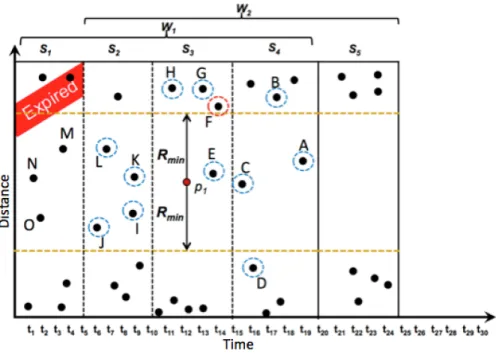
objects within a distance of rangerfor an object A, then A is classified as an outlier. For example, in Figure 1.1, if kis 4 andris fixed at a value, then an object A is regarded as an outlier if there are less than four objects within a distance of r from A (excluding A itself). It is not hard to check that objectsp8andp10are outliers based on the values ofk equal 4 andrequal R.
Figure 1.1: An Example of Distance-based Outliers
1.2
State-of-the-art Limitations
The problem of detecting outliers in streaming context has been studied in the literature [2, 17]. Both of them exploit computation on the overlap of sliding windows to avoid
huge overhead costs on computing from scratch at each window on the same data. [2] proposed a solution to detect outliers, whose number of neighbors are less thank within a distancer, in a count-based sliding windows while [17] proposed the solution for sup-porting outliers of the same definition in time-based sliding windows. [9] improves upon [2, 17] solutions by now supporting two additional distance-based outlier definitions (top n outliers with the highest distance and highest average distance to their respectivek near-est neighbors), and taking into account the temporal relationships among data points in streaming environment.
However, these existing techniques [2, 9, 17] did not consider the change of appropri-ate parameter settings over the streaming window. Moreover, they do not assist users in determining an appropriate parameter setting to detect the true outliers.
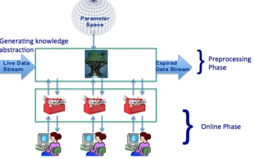
[8] proposed a methodology called ONION that enables analysts to effectively explore anomalies in large datasets. The platform consists of two phases: preprocessing phase to create the knowledge-based abstraction, which then supports the subsequent one, the phase of interactive online analytics. The preprocessing phase extracts and organizes the interrelationship among data. The online phase offers analysts several interactive tools to detect outliers with real-time responsiveness due to the support from the preprocessing phase.
This platform can be applied on dynamic datasets. However, there are disadvantages. The interactive operations will be delayed when there is new data because the knowledge-based abstraction needs to be updated. And, it will take approximately the same amount of time as the first preprocessing phase since there is no optimization applied in the context of dynamic datasets. As a result, its interactive analytics operations cannot be done with real-time responsiveness over dynamic datasets.
1.3
Challenges & Proposed Solution
Our goal is to offer a framework which enables interactive outlier exploration in streaming environment. As shown in Figure 1.2, as new data points keep coming, we preprocess them and build knowledge abstraction needed to support outlier exploration to analysts.
Figure 1.2: System Architecture
The first major challenge to achieve in detecting outliers in dynamic datasets is that detecting outliers in a single static dataset is already tedious because of the complexity of the algorithm. Thus, a streaming window adds more complexity on the task. Second, analysts need to supply a good parameter setting to yield the best result. So, acquiring an appropriate parameter setting is very important; yet, it is difficult to choose an appropriate one because the number of parameter setting is almost infinite. Last, the best parameter setting in one window is not guaranteed to be the best one in the other windows, because as data keeps evolving, the best parameter setting is also changing.
To address these challenges, we build a platform called Exploration Framework For Detecting Outliers In Data Streams (EFO) to support the outlier analytics tools of the
online phase of ONION framework in literature [8]. Our solution is to design, implement and evaluate an optimized technique for streaming environment. To do so, we design the preprocessing (offline) phase to handle data processing continuously while exploiting the previous execution as much as possible. Technically, we need to establish O-Space
andP-Spacefrom ONION offline phase and continuously update them when the window
moves.
First, a light-weight technique must be applied to overcome the performance bottle-neck of state-of-art methods in terms of CPU resource consumption. To achieve this goal, we should ideally focus on onlyoutlier candidates, those data points whose outlier status can change over data stream. We need to design a data structure to store necessary infor-mation of each outlier candidate when preprocessing them throughout the data stream. At the same time, we need to consider two optimization principles. One of the two principles namely ”best life expectancy,” is that we preprocess each data point by probing their re-spective neighbors in a reverse chronological time order because neighbors in the newest slide will survive longer or throughout the entire lifespan of the data point. The other principle called ”minimal trial,” leverages the first one by terminating the preprocessing of any data point which is found to hold stable outlier status as safe inlier, which will be explained in detail in Chapter 3. This approach constructsO-Space, the knowledge-based abstraction of ONION, efficiently in streaming environment.
Second, P-Spaceis built on top of O-Spaceto assist in choosing an appropriate pa-rameter setting which is likely to be changing across data stream. To establishP-Space, we need to build a number of outlier candidate lists ; each list corresponds to a value
k ∈ {kmin, kmax}, and stores all outlier candidates in increasing order of their respective
distance to kth nearest neighbor. The resulted lists reveal the parameter space as many regions; each region is calledstable region, which will always output the same result.
because of two major phenomena: (1) some outlier candidates can expire, and so do some of their respective neighbors (2) new arriving data points can be outlier candidates and can serve as the best neighbors for the remaining outlier candidates. Thus, an approach to update the outlier candidate lists and merge them with the new ones must be done con-tinuously. We observe that most of the lists are almost ordered so an incremental sorting technique called Ping Pong Patient Sort [11] is applied to leverage such phenomenon.
1.4
Contributions
For our EFO approach, we successfully tackled all challenges mentioned above. Contri-bution of our work on building this exploration framework to support outlier exploration over data stream are summarized as follows:
• We build a data structure with embedded personalized distance-threshold of each outlier candidate to store only necessary information throughout the streaming win-dow. The information is sufficient to support our platform and thus avoid huge overhead wasted on recomputing from scratch at each window.
• We apply intelligent time-aware preprocessing and safe inlier criterion in
establish-ingO-SpaceandP-Spacein streaming environment.
• We leverage almost-ordered outlier candidate lists in updatingP-Spacewith incre-mental sorting technique called Ping Pong Patient Sort.
• We validate the improved performance of our approach with experiments against the state-of-the-art ONION on two real datasets. The experimental study demon-strates significant improvement for a range of test scenarios of our proposed EFO platform.
The rest of the paper is organized as follows. Chpater 2 gives a brief introduction of the preliminary knowledge about Distanced-based Outlier Detection. The EFO platform is presented in Chapter 3. Experimental results are analyzed in Chapter 4. Chapter 6 covers related work, while Chapter 7 concludes the whole paper.
Chapter 2
Distanced-based Outlier Detection
Basics
2.1
Basic Concepts
An outlier is a pattern that does not conform to the expected behavior in a dataset. In recent years, several outlier definitions have been developed to separate outliers from the normal majority. One of the most widely used definitions is based on distance. In this work, we use the definition of distance-based outlier proposed in [16]. We use the term data point or point to refer to a multi-dimensional tuple. Let D be a set with n points
p1, p2, p3, ..., pn. The functiond(pi, pj)denotes the distance between data pointspiandpj
inD.
Definition 1 Given a dataset D, a range threshold r (r ≥ 0) and a count threshold k
(k ≥1), a pointpi ∈D is an outlier if fewer than k pointspj exist in D whose distance to
pi denoted asd(pi, pj)is not larger than r.
In order to understand the concept of EFO (Chapter 3), we need to define the follow-ing. In streaming database systems, we assume all arriving data points have their own
timestamp, denoted by pi.ts. If timestamp of pi is smaller thanpj, we mean that pi
ar-rives earlier thanpj on the input stream. For all neighbors ofpi whose timestamp is less
than timestamp of pi, we signify those neighbors as preceding neighbors of pi, denoted
as a set P(pi). Likewise, all neighbors of pi whose timestamp is larger than timestamp
of pi, we signify those neighbors as succeeding neighbors ofpi, denoted as a set S(pi).
Also, we have 4 input parameters: rmin, rmax, kmin, kmax; rmin and rmax are minimum
and maximum distance threshold respectively; kmin and kmax are minimum and
maxi-mum number of nearest neighbors respectively. r ∈ [rmin, rmax] is the range r which
plays an important role as the threshold to determine outlier status, as in Definition 1.
k ={kmin, kmin+ 1, ..., kmax−1, kmax}is another threshold in defining the outlier status
of any data point. The distance from a data pointpito itskmaxth nearest neighbor is denoted
asDkmax pi .
2.2
Outliers in Sliding Windows
One distinguishing trait of streaming data compared to static data is its infinity. In other words, data is always arriving in streaming systems on the fly. Keeping all these data is impossible in practice. Typically, analysis is conducted on fresh data instead of ancient ones as the new one interests us and has more immediate relevance and thus value hid-den. Therefore, sliding window semantics, widely used in the literature [23, 2], not only separate infinite data into finite snapshots, but also enable us to overcome the difficulties caused by the continuity of data stream. We have adopted these semantics, which are used in our algorithm.
We work with periodic sliding window semantics as proposed by CQL [3] for defin-ing the sub-stream of interest from the otherwise infinite data stream. Sliddefin-ing window semantics can be either time based or count based. Each window W has a fixed window
sizeW.winand slide sizeW.slide. For time-based windows, each windowW has a start-ing timeW.T startand an ending timeW.T end =W.T start+W.win. Periodically, the current window W slides, causing W.T start andW.T end to increase by W.slide. For count-based windows, a fixed number (count) of data points corresponds to the window sizeW.win. The window slides after the arrival ofW.slidenew data points.
Assumptions. Other factors besidesr,k,W.win, andW.slidecould be adjusted, such as the distance function and higher dimensional data. The distance function used to compute pair-wise distances is quite flexible. As long as the distance function is meaningful, any distance function could be used as a metric for outlier mining. Here, we make the assump-tion that our algorithm uses Euclidean distance as the metric with a fixed dimensionality. The parameters that can be altered arer,k,W.win, andW.slide.
Chapter 3
EFO Framework
EFO platform is designed to handle data preprocessing in streaming environment to sup-port ONION operations in the online phase of literature [8]. EFO continuously prepro-cesses data points over streaming window while exploiting the previous execution to es-tablishO-SpaceandP-Spacefrom ONION offline phase, and continuously update them when the window moves. Thereafter, it will support two outlier exploration operations: Outlier Detection and Outlier-centric Parameter Space Exploration.
To begin, we need to understandO-SpaceandP-Space. Thereafter, we will demon-strate the approaches to realizeO-SpaceandP-Spacein the streaming context. Then we will show how they support the outlier exploration operations.
3.1
O-Space
Let us review O-Space from literature [8]. O-Space is a three-dimensional space that models the distribution of the outliers with respect to their associated parameter settings.
Definition 2 and Lemma 1, 2, 3, and 4 are taken from the literature [8].
space with the possible settings of parameters r, k and data points p in dataset D be-ing its three dimensions. The dimensionDimkranges over the values that the parameter
k can take in the universe of natural number Uk : [kmin , kmax], wherekmin and kmax
are the user-specified lower and upper bounds of the k values. Similarly, the dimension
Dimr corresponds to the domain of real numbersUr : [rmin , rmax] withrmin andrmax
the lower and upper bounds of the values of parameter r. Lastly the dimension Dimd
represents all points p∈D sorted into a linear order. Each point is assigned a position in [1,|D|]. Each coordinate (ki,ri,pi )∈OSmaps to a boolean value v∈ {0,1}indicating
whether pointpiis an outlier with respect to parameter valueski andri.
In this O-Space, any combination of k and r values on the dimensions Dimk and
Dimr forms a parameter setting psi denoted by psi (ki , ri). Conceptually, O-Space
encodes the outlier status of all points inDwith respect to all possible parameter settings. Since dimension Dimd represents all data points in dataset D, Dimd corresponds
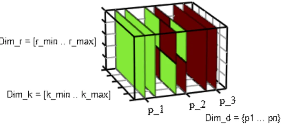
to a discrete domain of positions. In other words, the three-dimensional O-Space can be thought of as a sequence of two dimensional slices formed by the dimensions Dimk
andDimr, as shown in Figure 3.1. Each slice models the outlier status distribution with
respect to all possible parameter settings for one particular pointpiin datasetD. The green
color represents inliers, and the brown color represents outliers. So, the green slices mean their corresponding data points are inliers for all parameter settings; the brown slices mean their corresponding data points are outliers for all parameter settings; and, the mixed-color slices mean their corresponding data points are inliers for some parameter settings and outliers for the other parameter settings.
O-Spacedepends on following foundations, taken from the literature [8], to efficiently establish insights based on the two dimensional subspacesDimkandDimr.
Lemma 1 Given a set of parameter settings Pk ⊂ P, where ∀ two parameter settings
Figure 3.1: O-Space Visualization
any psx inPk is determined by the distance between pi and its kth nearest neighbor pj
denoted asDk pi.
Proof. Given any parameter settingpsx(k,rx)∈ Pk, ifDkpi > rx, then by the definition of
the kth-nearest neighbor, there are at most k-1 other pointspj∈Dwhose distance towards
pi is not larger than rx. In other words, pi has at most k-1 neighbors. By Definition
1, pi is an outlier. On the other hand, if Dpik ≤ rx, then there are at least k points pj
with d(pi,pj) ≤ rx, namely pj are all neighbors ofpi. pi is then classified as an inlier
by Definition 1. Therefore ∀ psx(k,rx) ∈ Pk, the outlier status of pi can be correctly
determined by comparingrxagainstDpik. Lemma 1 is proven.
Lemma 2 A pointpi is a constant inlier ifDpikmax ≤rmin.
Proof. If the distance to pi’skmaxth nearest neighbor is ≤ rmin, thenpi has at leastkmax
neighbors or more even under the most restricted neighbor criteria, namelyDimr=rmin.
Thenpi is an inlier forps(kmax,rmin) that is the most restricted parameter setting inP in terms of recognizing outlier. Ifpi is not an outlier in the most restricted setting, then of
course it cannot be an outlier in any part ofP. Thereforepiis a constant inlier.
Proof. Lemma 3 can be proven in the similar way of proving Lemma 2. If the distance to
pi’skminth nearest neighbor is> rmax, thenpihas at mostkmin−1neighbors under the least
restricted neighbor criteria, namelyDimr =rmax. Thenpi is an outlier forps(kmin,rmax)
that is the least restricted parameter setting inP in terms of recognizing inlier. Ifpiis not
an inlier in the least restricted setting, then of course it cannot be inlier in any part ofP. Thereforepi is a constant outlier.
The idea of constant inlier and constant outlier here is in the context ofstatic dataset. We will see how they exist in thestreaming contextlater in Section 3.1.1.
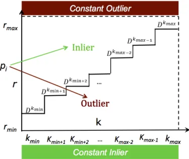
Figure 3.2: Space Delimiter
Lemma 4 Given a dataset D and parameter setting space P, ∀pi ∈D the distance set
DS(pi)={Dpkix|kmin ≤kx ≤kmax}is sufficient to determine the outlier status of pi with
respect to any parameter setting ps∈ P.
Proof. P = Pkmin ∪ Pkmin+1 ∪ Pkmin+2 ... ∪ Pkj ... ∪ Pkmax−1 ∪ Pkmax, where Pkj is
composed by anypsx(kx, rx)∈ P withkx =kj (kmin ≤kj ≤kmax). Therefore given any ps ∈Pps is guaranteed to be covered by somePkj. By Lemma 1,∀ps ∈ Pkj the status
of pi can be determined by examining D kj
pi. Since D kj
pi ∈ DS(pi), therefore DS(pi) is
sufficient to determine the status ofpiwith respect to anyps ∈ P. Lemma 4 is proven.
As shown in Figure 3.2 this distance setDS(pi)delimits P into two segments. The
parameter settings in different segments will classifypito different outlier status.
There-foreDS(pi)is calledspace delimiterofpi. The set of space delimiters{DS(pi)|pi ∈D} effectively represents the three dimensionalO-Space.
Since any data points that are found to be constant inliers and constant outliers, their outlier status will never change. Thus, only data points found to be outlier candidates are necessary to maintain their respective space delimiter.
3.1.1
O-Space Construction in EFO
The key idea behind buildingO-Spaceis basically findingkmaxnearest neighbors of each
data point to reveal outlier status and store space delimiter of only outlier candidates. In streaming environment, to establish O-Space efficiently, we need to utilize two major principles: Best Life Expectancy andMinimal Trial (Safe Inlier). In addition, we need to build a data structure to store necessary information (space delimiter)of outlier candidates over the data stream.
Best Life Expectancy
Lemma 5 Given a data point pi arriving at time stamp pi.ts and its two neighborspj
with pj.ts and pk with pk.ts , if both pj and pk have the same distance from pi , and
pj.ts < pi.tswhilepk.ts ≥pi.ts thenpk has best life expectancy to serve as the nearest
neighbor, compared topj. So,pkis maintained instead ofpj.
Proof. This principle utilizes the fact that the data point pk which arrived later in the
window are guaranteed to have a more decisive impact compared to the earlier data point
pi , and it will persist throughout the whole lifespan ofpi. As shown in Figure 3.3, there
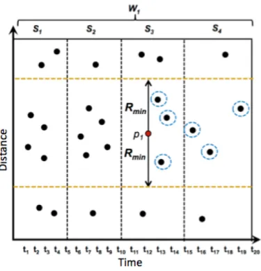
are two groups of neighbors for p1. They are both potential neighbors for p1 in term of distance top1. The difference between them is the arrival time. The first group arrives in slideS1while the second group arrives in slideS4. Assume the window moves one slide at a time; so, when it moves fromW1 toW2, the group inS1 expires while the group in S4 is still in the window. When it moves again, fromW2 toW3, the neighbors inS4 has not expired yet, and thus serve asp1’s neighbors throughout its entire lifespan.
Figure 3.3: Best Life Expectancy Of Neighbors For An Outlier Candidate
This principle will identify the most lasting neighbor relationships of each outlier candidate which are used to build the space delimiter. So, in probing nearest neighbors for a data point, we start from the latest slide in the window to the earliest ones to avoid storing unnecessary information.
Lemma 6 Given a data pointpi, if size ofS(pi)≥kmaxand at leastkmaxpoints ofS(pi)
whose respective distance topiare≤rmin, thenpi is a safe inlier.
Proof. For a data pointpi, if itskmaxnearest neighbors in succeeding slide already satisfy
the most restricted thresholdrmin, thenpiis guaranteed to be inlier over its entire lifespan
because all of its kmax nearest neighbors will not expire beforepi itself. This meanspi
will never become an outlier at any time. For example as shown in Figure 3.4, assume thatkmax = 4, thenp1 is considered asafe inlierbecause it has more than four neighbors in its succeeding slides (S3andS4) and these neighbors are within the restricted distance thresholdrminfromp1.
Figure 3.4: Safe Inlier
Unlike instatic dataset, there is neither constant outlier nor constant inlier. Instead, safe inlieris the only special status identifying that a data point is always an inlier during its entire lifespan, which is equal to constant inlier in static dataset. As long as a data
point pi satisfies thesafe inlier condition, the probing operation on pi is terminated and
then move on to another data point. Thus,safe inlier leverages the order of probing from the latest slide to the earliest slide because it can avoid unnecessary computation wasted on probing in preceding slides.
Data Structure
We build a data structure to store necessary information. A nodenis the data structure composed of the following elements:
• n.id: the identifier of the object, that is the arrival time of the object;
• n.nn s: a list of (kmax−kmin) neighbor lists in each slide of the window;
• n.nn suc: a list ofkmaxnearest neighbors inpi’s succeeding slide;
• n.dist: a distance value frompitokmaxnearest neighbors in its succeeding slide;
• n.nn g: a list of globalkmax nearest neighbors in the window.
Each list stores the neighbors by the order of itskminth neighbor at the head and the
kthmaxneighbor at the end.
3.1.2
A Running Example of O-Space Construction in EFO
Initial Preprocessing. First, we start with a preprocessing phase that processes the
in-coming data points in an intelligent time-aware order. That is, to find neighbors for each data pointpi, we probe from succeeding slides to preceding slides. For any data pointpi
that is an outlier candidate, we will store necessary information to avoid the computation from scratch for the same data points every time the window moves.
For the following step-by-step example, assume we have data points laid out as shown in Figure 3.5. Supposekmax = 4andrmin = 5. Forp1 , we store:
• kmax nearest neighbors in each slide of the window (p1.nn s): S4: A, B, C, D
S3: E, F, G, H S2: I, J, K, L S1: M, N, O
S1stores only these three neighbors because the other data points do not satisfy the personalized distance-threshold of p1: p1.dist. This approach reduces the number of unnecessary neighbors to maintain because those unnecessary neighbors will not be a part of the space delimiter ofp1 throughout its entire lifespan.
• kmax nearest neighbors inp1’s succeeding slide (p1.nn suc): A, C, E, F
• Distance fromp1tokmaxnearest neighbors in its succeeding slide (p1.dist): 5.1 (assumed(p1, F) = 5.1; sop1.dist= 5.1because F is thekmaxth nearest neighbor
in succeeding slides.)
• Globalkmaxnearest neighbors ofp1in the window (n.nn g): C, E, K, N
Continuously Preprocessing. Assume the window moves one slide at a time as shown
in Figure 3.6. So, when the window moves from W1 to W2, the data points in slide S1 expire while there are new arriving data points in slideS5. We need to preprocess the new arriving data points and update the non-expired ones.
For new arriving data points in slideS5, we simply need to follow the same step in
Initial Preprocessingphase.
For each non-expired data point, for examplep1 that is in slideS3, there are 3 steps to process. First, we remove the information ofS1because it is already expired. Second,
Figure 3.5: Initial Preprocessing
we need to find its nearest neighbors in the new slideS5. As seen in Figure 3.6, there is no need to store any neighbor in slideS5 because none of the data points inside slideS5 satisfiesp1’s personalized distance-thresholdp1.dist, which isd(p1, F). Third, we need to re-computep1’s globalkmaxnearest neighbors by merging the neighbors maintained in
each slide of the current window (now isW2).
Thus, for continuously preprocessing p1 , we update the information maintained as follows:
• kmax nearest neighbors in each slide of the window (p1.nn s): S4: A, B, C, D
S3: E, F, G, H S2: I, J, K, L S5: ∅
Figure 3.6: Continuous Preprocessing
satisfies the personalized distance-threshold ofp1: p1.dist. Again, we see that this approach saves memory resource by not maintaining unnecessary neighbors in the latest slide.
• kmax nearest neighbors inp1’s succeeding slide (p1.nn suc): A, C, E, F
• Distance fromp1tokmaxnearest neighbors in its succeeding slide (p1.dist): 5.1
Since data point F is still thekth
maxnearest neighbor in succeeding slides, there is no
update on the distance-thresholdp1.dist.
• Globalkmaxnearest neighbors ofp1in the window (n.nn g):
C, E, K, A (because A is the closest neighbor top1after C, E and K)
now S5 has a data point X which satisfies the personalized distance-threshold ofp1, and so X must be maintained. Moreover, thekmax nearest neighbors inp1’s succeeding slide must be updated to C, E, A, and X (the kthmax nearest neighbor F is now replaced by X). Since each distance from C, E, A, and X top1 respectively is less thanrmin,p1 becomes
safe inlier which is thus no more needed to be maintained.
Figure 3.7: A Data Point BecomeSafe InlierOver Data Stream
3.1.3
Outlier Detection Supported by EFO O-Space
So now that we can maintain the O-Space, technically thespace delimiters of all outlier candidates over the data stream, we can support Outlier Detection operation in a streaming environment.
As explained in Running Example Section 3.1.2, for each outlier candidate oc we maintain its space delimiter DSin an array structure by the order of itskth
min neighbor at
the head and the kth
outlier status ofoccan be immediately determined by applying the followingexamination rulefrom literature [8].
Definition 3 Given an outlier candidate oc and its DS structure, ∀ parameter setting ps(kx,rx)inP,ocis an outlier ifDS[kx−kmin]>rx. Otherwiseocis an inlier.
Therefore to answer Outlier Detection, we only need to sequentially apply the exami-nation rulein Definition 3 on eachoc.
3.2
P-Space
Now let us review P-Space from literature [8]. P-Space represents the whole possible parameter settings in a form of a finite number of parameter regions which reveal rela-tionships among outlier candidates and the insight of how changes in parameter settings may impact the resulting outliers.
Definition{4, 5}and lemma{7, 8, 9}are taken from literature [8].
Definition 4 P-Space denoted asP=P1 S
P2 ... SPm, such that:
(1) given any two parameter setting subsetsPi andPj ofP(1≤i, j≤m),PiTPj =∅;
(2) given any two parameter settingspsj andpslin the samePi (1 ≤i ≤m),psj andpsl
generate the same set of outliers.
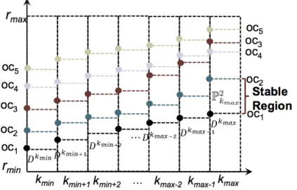
In other words P-Space divides the two-dimensional space formed by the set of all possible values on the Dimk, Dimr axes into a set of disjoint regions. These region are formed byspace delimitersof all outlier candidates fromO-Spaceat eachkvalue of di-mensionDimk, as shown in Figure 3.8. Within each region no matter how the parameter
settings are adjusted, the set of outliers generated from dataset D remains unchanged. Each such region is called astable region, also shown in Figure 3.8.
Figure 3.8: P-Space and Stable Region
P-Spacefurther reveals relationships among outlier candidates through the concept of
k-dominationbetween two outlier candidates.
Definition 5 Given two outlier candidatesociandocjand a valuekofDimk ∈[kmin,kmax], ifDk
oci 6D
k
ocj, thenocik-dominates ocj .
The followingmonotonic propertyholds if the k-domination relationship holds be-tweenociandocj.
Lemma 7 Given two outlier candidates oci andocj withoci k-dominatingocj, then for
any parameter settingps(k,rx)∈ P (rmin ≤rx ≤rmax), ifoci is classified as outlier by
ps, thenocj is guaranteed to be outlier with respect tops.
Proof. Ifoci is an outlier with respect tops(k,rx),Docki >rx. SinceD
k
ocj ≥D
k
oci by the
k-domination definition in Definition 5,Dk
ocj >rx. Thereforeocj is an outlier with respect
tops.
In other words, if one parameter settingps(k,rx)classifiespi as an outlier, then any
parameter setting classifies pi as an inlier, then any point that k-dominates pi is also
guaranteed to be an inlier as well.
It is straightforward to prove that the k-domination relationship also satisfies the transitive property.
Lemma 8 Given three candidates och, oci, and ocj, if och k-dominates oci and oci
k-dominatesocj, thenochk-dominatesocj.
Proof. Since och k-dominatesoci, Dockh ≤D
k oci. Similarly D k oci ≤ D k ocj, because oci k-dominatesocj. ThereforeDockh ≤D k
ocj , which meansoch k-dominatesocj by Definition
5.
The above properties of thek-dominationrelationship now enable us to divide the infinite parameter setting spaceP into a finite number ofstable parameter regions. Lemma 9 Given the outlier candidate setOC⊂dataset D andPki ⊂ P, where|OC|=
n andPki is composed by any parameter setting ps inP sharing the sameDimkvalueki,
thenPki can be divided into n+1 stable regionsPjki , whereDimr ofPki1 ∈[rmin,Docki1),
Dimr of P2ki ∈ [Docki1,D ki oc2), ..., Dimr of P j+1 ki ∈ [Dockij,D ki ocj+1) ,...., Dimr of P n+1 ki ∈ [Dki ocn,rmax](D ki oc1 <D ki oc2, ...,<D ki ocj <D ki ocj+1, ...,<D ki
ocn). The identical set of outliers
are guaranteed to be generated for all ps∈Pjki.
Proof. ∀ps(ki,rx)∈Pkij , sinceDockij−1 ≤rx <D
ki
ocj, ps(kj,rx)will classifyocj−1 as
in-lier, while ocj would be classified as outlier. Since Dockij−2 <D
ki ocj−1 andD ki ocj <D ki ocj+1,
we getocj−2 k-dominatesocj−1 andocj dominatesocj+1. Based on the monotonic prop-erty of k-domination, ocj−2 will also be classified as an inlier, while ocj+1 remains as outlier. Furthermore by the transitive property of k-domination, ∀ ps(ki,rx) ∈ Pkij+1,
oc1,oc2, ...,ocj−2,ocj−1 are guaranteed to be inliers, whileocj,ocj+1, ...,ocn are guaran-teed to be outliers. Therefore the identical set of outliers will be generated for anyps ∈ Pjki+1. Lemma 9 has thus been proven.
As explained so far, P-Space models the infinite input parameter space into a finite number of stable regions which respectively contain a large range of continuous parameter settings that generates the same set of outliers.
In short,P-Spaceis basically built uponO-Spaceusingspace delimiters. Technically, it is represented by m = (kmax −kmin+1) lists; each list called kthList contains all outlier candidates sorted (in ascending order) based on their distance to theirkth nearest
neighbors with respect to each k from kmin to kmax. Therefore, each outlier candidate
ocis represented exactly once in eachkthList. Then for example, the parameter settings between the Dkmax of oc1 and oc2 (denoted asP2kmax) is a stable region. All parameter
settings in this region will classifyoc4,oc3 andoc5 as outliers, as shown in Figure 3.8.
3.2.1
P-Space Construction in EFO
The key idea behindP-Spaceis to sort all outlier candidates in eachkthListin ascending order based on their distance to theirkthnearest neighbors.
Similar tostatic dataset, to establishP-Spacein streaming environment we first need to build each kthList which corresponds to each k from kmin to kmax. This can be
realized by scanning m = (kmax −kmin +1) times over the outlier candidate set OC. For each scan, we put each outlier candidate oc into corresponding kthList, and sort them based on their distance to theirkthnearest neighbors.
When the window moves, there are some phenomena related to outlier candidatesoc; some oc can expire; some others can become safe inliers; also, there can be some new outlier candidates from the latest slide. This means that P-Space changes over sliding window. This is a very important procedure in establishing P-Spacein streaming envi-ronment. With that said, to efficiently updateP-Space, we need to follow three steps.
• Remove from eachkthListany outlier candidateocwhich expired in the new win-dow (the current one) or which became asafe inliers.
• Update eachkthListaccording to any remaining outlier candidateocwhose global
kmax nearest neighbors changed.
We call the kthListlists that we just updated, theOld Lists. In updating theOld Lists, we observe that even though some outlier candidates expire after the window moves, all of the remaining outlier candidates in each kthListof the Old Lists is in almost sorted order. Thus, we use an incremental sorting technique called Ping Pong Patient Sort in literature [11], to exploit the nature of such almost sorted lists.
• Build atemporarykthListlists containing new outlier candidates in the latest slide and then merge them with the correspondingkthListof theOld Lists.
Therefore, we obtain the updatedkthListlists, which serve asP-Spaceof the cur-rent window.
3.2.2
A Running Example of P-Space Construction in EFO
Initial Preprocessing. P-Spaceis built uponO-Space. As shown in Figure 3.9, suppose
there are five outlier candidates (oc1, oc2, oc3, oc4, oc5) in current window calledW1. For this first window, EFO simply builds each sorted kthListlist by using the global kmax
nearest neighbors of each outlier candidate.
To simplify the example, let’s focus on onlykthListofkminandkmax, calledkthListkmin
andkthListkmax respectively. Thus, the resultedP-Spacewill be as follows.
• kthListkmin:oc1, oc2, oc3, oc4, oc5. • kthListkmax: oc1, oc2, oc4, oc3, oc5.
Continuously Preprocessing. When the window moves to the next one calledW2, some
data points expire including outlier candidates and their neighbors while some new data points arrive. So, there must be change in kthList lists from W1, now called the Old
Figure 3.9: EachkthList’s Representation In WindowW1
kthList Lists as shown in Figure 3.10. Also, there can be new outlier candidates in the latest slide ofW2that we need to maintain in the form oftemporarykthListlists, shortly called the New kthList Lists, as shown in Figure 3.11. For the Old kthList Lists, since
oc5 expires (does not exist inW2), then we need to update the outlier candidate lists by removing oc5 from eachkthList. As seen that the distance to kthmin nearest neighbor of
oc4 now changes to locate betweenoc2 andoc3, and the distance tokthmaxnearest neighbor
ofoc2 changes to the greatest distance among remainingocinkthListkmax. So, we need
to update bothkthListkmin andkthListkmax accordingly.
Therefore, we obtain the updatedOld kthList Listsas follows.
• kthListkmin:oc1, oc2, oc4, oc3. • kthListkmax: oc1, oc4, oc3, oc2.
For theNew kthList Lists, there are two new arriving outlier candidates: oc6 and oc7 as in Figure 3.11. Thus, we build the temporarykthListlists as follows.
Figure 3.10: The OldkthList’s Representation In WindowW2 • kthListkmin:oc6, oc7.
• kthListkmax: oc7, oc6.
Finally, by merging the Old kthList Lists and New kthList Lists we get the updated P-Spaceas in Figure 3.12. The updatedkthListlists are as following.
• kthListkmin:oc1, oc2, oc4, oc3, oc6, oc7. • kthListkmax: oc1, oc4, oc3, oc7, oc2, oc6.
Incremental Sorting. Behind the scene to obtain the updatedOld kthList Lists, we utilize
an incremental sorting technique called Ping Pong Patience Sort [11]. From our obser-vation, most of kthListlists are almost ordered so the incremental sorting technique is applied to leverage such phenomenon.
For example, let’s look at only onekthList ofkmin. Assume thekthListkmin
Figure 3.11: The NewkthList’s Representation In WindowW2
oc oc1 oc2 oc3 oc4 oc5 oc6 oc7 oc8 oc9 oc10 oc11 oc12 Dkmin
oc 1 2 3 3 4 4 5 5 5 6 7 8
Table 3.1: kthListkmin: Outlier Candidates With Distance to TheirkminNearest Neighbor
oc1, oc5, oc6,andoc7 expired, whileDkminoc4 andD
kmin
oc8 changed to 4 and 2 respectively, as
in Table 3.2. If we take out the two updatedoc4andoc8, and append them at the end of the list, we see thatkthListkmin is an almost sorted order, as in Table 3.3. Instead of sorting
the list from scratch, we exploit its almost sorted nature using incremental sorting called Ping Pong Patience Sort.
To give a summary of how Ping Pong Patience Sort works, we can sortkthListkmin
from Table 3.3 as an example. First, we need to build sorted runs. A sorted run is a sorted list of elements from the main list. At the begining, there are no sorted runs, so a new
oc oc2 oc3 oc4 oc8 oc9 oc10 oc11 oc12 Dkmin
oc 2 3 4 2 5 6 7 8
Figure 3.12: The MergedkthList’s Representation In WindowW2 oc oc2 oc3 oc9 oc10 oc11 oc12 oc4 oc8 Doc
kmin 2 3 5 6 7 8 4 2
Table 3.3: kthListkmin: An Almost Sorted List
sorted run is created to insert 2. Since 3 comes after 2, it is added to the end of the first run. Similarly, 5 is added to the first run and so do 6, 7 and 8. Since 4 cannot be added at the end of the first run, a new run is created with 4. Since the last element 2 cannot be added to either the first or second sorted run, a third sorted run is created for 2. We finally obtain three sorted runs as in Figure 3.13. Next, we pack all sorted runs together in order of the size of each sorted run as in Figure 3.14. Last, we always merge the 2 sorted runs with smallest size at a time as in Figure 3.15.
Figure 3.13: Sorted Runs
Figure 3.14: Pack Sorted Runs
Figure 3.15: Merge Runs (Smaller To Larger)
3.2.3
Outlier-Centric Parameter Space Exploration Supported by EFO
P-Space
Outlier-Centric Parameter Space Exploration is the operation from ONION online phase in [8] that offers analysts the insight of stable regions, which let them know how changes in parameter settings may impact the resulting outliers.
As explained in Running Example Section 3.2.2, we can maintain theP-Spaceover the data stream, technically eachkthListlist corresponding to eachkfromkmintokmax.
For each window Wi we maintain each up-to-date kthList list which stores all outlier
candidates in ascending order of distance to correspondingk. It offers the insight ofstable region which partitions the infinite possible parameter settings into a finite number of parameter setting space. Within each stable regionno matter how the parameter settings are adjusted, the set of outliers generated from the same window remains unchanged. More specifically, given a stable region Pjki: [Dki
ocj−1, D
ki
ocj), it will generate ocj, ocj+1,
...,ocn as outliers, namely the points listed behindocj−1 with respect to its lower bound Dki
ocj−1.
[8] as following.
Definition 6 PSE. Given an outlier set Oin and aδ (−1 < δ <1) as input, report all
parameter settingspsj ∈P-SpaceP, such that:
(1) ifδ≥0,psj identifies an outlier setOj ⊆Oinwhere|Oj |= (1 -δ)|Oin|;
(2) ifδ≤0,psj identifies an outlier setOj ⊇Oinwhere|Oj |= (1 -δ)|Oin|.
PSE leverages the stable region property of P-Space and allows analysts to conve-niently evaluate the stability of a given outlier set Oin. This is one important indicator
of how significant the observed abnormal phenomena is. For example, if we set theδ as 0, PSE will return all the parameter settings that are guaranteed to generate the outliers identical toOin, namely a stable region ofP. The scope of the returned parameter settings (the size of the stable region) represents how stable the outlier set is acrossP-Space.
Furthermore, PSE provides a tool for analysts to examine how changes in parameter settings may impact the resulting outliers. PSE achieves this, for example, by allowing the analysts to apply PSE to ask for the parameter settings that would return around (1 - δ)% of Oin as the results, and then compare them against the parameter settings that
Chapter 4
Performance Evaluation
4.1
Experimental Setup
Our proposed EFO platform is implemented using Java on CHAOS Stream Engine [14]. The experiments are conducted on a PC with Intel Core i7 CPU 3.40 GHz (4 Cores) and 8 GB RAM, which runs Windows 7 OS.
Real Datasets. We use two real streaming datasets. Dataset 1 is the Moving Target Indicator (GMTI) from MITRE Corporation, and Dataset 2 is the Stock Trading Traces dataset (STT) from NYSE. Except timestamp, both datasets are in two dimensions. GMTI contains 45,000 records of real moving objects observed in a certain area of location within six hours. STT has one million transaction records throughout the trading hours of one day.
Metrics. We measure two common metrics for stream systems, namely CPU time and average memory consumption. CPU time corresponds to the total amount of the system time used to preprocess the whole data stream. The consumed memory corresponds to average memory required to store the information throughout the whole data stream. All experiments are performed using count-based mechanism, and window moves one slide
at a time.
Alternative Algorithms. Our experiment focuses on the performance of EFO against the state-of-the-art ONION for preprocessing phase.
Methodology. We evaluate the performance of the proposed approach by varying the most important parameters. Specifically, our experiments cover the three major cost factors, namely stream volume, velocity, and outlier rate. We measure scalability on high volume streams by varying thewindow sizewhile leaving all other settings constant. We also vary the velocity of a data stream by varying the slide size while leaving all other settings constant. Similarly, we measure how well these methods work for different outlier rates. For the distance-threshold type, this means varying rmin , while for kN N
type it means varyingkmax.
4.2
Varying Window Size Evaluation
We first analyze the effect of stream volume by varying the window size while leaving all other settings constant. Window size refers to the number of data points per current window that the preprocessing task is focusing on.
GMTI Experiment. We varywindow sizefrom 1,000 data points per window to 10,000 data points per window. We choose arbitrary fixed value for other settings rmin =
0.1, rmax = 0.5, kmin = 1, kmax = 10, and slidesize = 200. We observe how EFO
and ONION perform when the volume of data streams gets higher and higher.
Figure 4.1 shows the processing time of both approaches on Y-axis and window size on X-axis. As can be seen, both EFO and ONION perform similarly for small window sizes. Yet, EFO outperforms ONION as the window size gets larger. When
windowsize = 4,000 , the processing time of EFO is as low as smaller window sizes while ONION takes approximately 2.5 times of EFO. As the window size gets bigger at
windowsize = 10,000, EFO outperforms ONION up to approximately 9 times. This is because ONION preprocesses each window from scratch while EFO always lever-ages preprocessing from previous windows. With that said, the bigger the window size, the more data points ONION needs to preprocess from scratch at each window. Unlike ONION, the bigger the window size, the less data points EFO needs to preprocess com-pared to ONION.
Figure 4.2 shows the average memory usage of the two approaches for varying win-dow size. Y-axis is used as measurement of memory inKBs, and X-axis again shows the varying window sizes. Both EFO and ONION consume very similar memory for smaller window size. Yet, as expected, EFO consumes more memory than ONION when the window size gets larger and larger. This is because the larger the window size, the more information (technically equivalent to the more slides) EFO needs to store throughout the data stream while ONION needs to store only information of outlier candidates in each window. The trends of both EFO and ONION are increasing logically because the bigger the window size, the more information (data points) they maintain.
Figure 4.1: Varying Window Size on GMTI CPU Processing Time
Figure 4.2: Varying Window Size on GMTI Memory Consumption
STT Experiment. We now conduct experiment on STT dataset by varyingwindow size from 1,000 data points per window to 10,000 data points per window. We choose arbi-trary fixed value for other settings rmin = 0.001, rmax = 0.5, kmin = 1, kmax = 5, and
slidesize = 200. We observe how EFO and ONION perform when the volume of data streams gets higher and higher.
Figure 4.3 shows the processing time of both approaches on Y-axis and window size on X-axis. As shown, both EFO and ONION perform similarly atwindowsize = 1000. Yet, EFO outperforms ONION as the window size gets larger. When windowsize = 10,000 , the processing time of EFO is approximately 7 times faster than ONION. The reason is the same to GMTI dataset. That is, ONION preprocesses each window from scratch while EFO always leverages preprocessing from previous windows. With that said, the bigger the window size, the more data points ONION needs to preprocess from scratch at each window compared to EFO.
Figure 4.4 shows the average memory usage of the two approaches for varying win-dow size. Y-axis is used as measurement of memory inKBs, and X-axis shows the varying window size. As depicted, at smaller window sizes (between 1,000 to 3,000), EFO con-sumes slightly more amount of memory from ONION but as window size gets larger, it consumes more and more memory compared to ONION. This is as expected because the bigger the window, the more information to store because of more data points, in addition to the fact that EFO store more information than ONION for an outlier candidate.
Figure 4.3: Varying Window Size on STT CPU Processing Time
Figure 4.4: Varying Window Size on STT Memory Consumption
4.3
Varying Slide Size Evaluation
We now analyze the effect of velocity of the data stream by varying theslide size while leaving all other settings constant. Slide sizerefers to the number of data points per slide. The window moves after the arrival of new data points equal toSlide size.
GMTI Experiment. We vary slide size from 500 data points per slide to 5,000 data points per slide. We choose arbitrary fixed value for other settings rmin = 0.1, rmax =
0.5, kmin = 1, kmax = 10, windowsize = 20,000. We observe how EFO and ONION
perform when the slide size gets larger and larger.
Figure 4.5 shows the processing time of both approaches on Y-axis and varying slide sizes on X-axis. As can be seen, EFO outperforms ONION at any slide size. When
slidesize = 500, the processing time of EFO wins over ONION for approximately 13 times. The larger the slide, the less windows over the data stream that both approaches need to preprocess. This is the reason why the trends of both approaches are decreasing. Again, EFO outperforms ONION because EFO leverages preprocessing from previous windows while ONION preprocesses each window from scratch over the data stream.
Figure 4.6 shows the average memory usage of the two approaches for varying slide size. Y-axis is used as memory consumption in KBs, and X-axis shows the varying slide sizes. As expected, EFO consumes more memory than ONION because of stor-ing the information from previous windows to leverage time consumption on preprocess-ing. ONION consumes memory approximately the same because varying slide size does not increase the number of data points per window, unlike varying window size. Unlike ONION, per outlier candidate, EFO needs to store extra information (multiple kthList
lists for each slide) in addition to its global kmax nearest neighbors. This is the reason
why it consumes more memory than ONION. Yet, EFO memory consumption improves as the slide get bigger. The reason is because the bigger the slide size, the less number of
slide per window. Thus, per each outlier candidate EFO needs to store lesskthListlists over the data stream.
Figure 4.5: Varying Slide Size on GMTI CPU Processing Time
Figure 4.6: Varying Slide Size on GMTI Memory Consumption
STT Experiment. We varyslide sizefrom 500 data points per slide to 5,000 data points per slide. We choose arbitrary fixed value for other settings rmin = 0.001, rmax =
0.5, kmin = 1, kmax = 5,andwindowsize = 20,000. We observe how EFO and ONION
perform when the slide size gets larger and larger.
Figure 4.7 shows the processing time of both approaches on Y-axis and varyingslide size on X-axis. As can be seen, EFO outperforms ONION at any slide size. When
slidesize = 500 , the processing time of EFO wins over ONION for approximately 8 times. The larger the slide, the less windows over the data stream that both approaches need to preprocess. This is the reason why the trends of both approaches are decreasing. Technically again, EFO outperforms ONION because EFO leverages preprocessing from previous windows while ONION preprocesses each window from scratch over the data stream.
Figure 4.8 shows the average memory usage of the two approaches for varying slide size. Y-axis is used as memory consumption in KBs, and X-axis shows the varying slide sizes. We see that the result is consistent with GMTI dataset because the larger the slide, the less number of slide per window which is why EFO trend is decreasing while ONION
have little variation in memory consumption.
Figure 4.7: Varying Slide Size on STT CPU Processing Time
Figure 4.8: Varying Slide Size on STT Memory Consumption
4.4
Varying
k
maxEvaluation
We now compare EFO and ONION for different outlier rates based onkNN type, which means varyingkmaxwhile leaving all other settings constant.
GMTI Experiment. We varykmax from 5 neighbors to 45 neighbors. We choose
arbi-trary fixed value for other settings rmin = 0.1, rmax = 1.5, kmin = 1, windowsize =
20,000,andslidesize = 500. We observe how EFO and ONION perform when outlier rate increases.
Figure 4.9 shows the processing time of both approaches on Y-axis and varyingkmax
on X-axis. As depicted, EFO outperforms ONION as outlier rate increase. Whenkmax =
5 , the processing time of EFO outperforms ONION for approximately 9 times. Both approaches consume more time askmax increases, basically because the biggerkmax, the
more neighbors they need to probe for each data point. Also, this is the reason why EFO continues to win over ONION when kmax increases since EFO save much computation
instead of recomputing from scratch in probing many (kmax) nearest neighbors in each
Figure 4.10 shows the average memory usage of the two approaches for varyingkmax.
Y-axis is used as memory consumption inKBs, and X-axis shows the varyingkmax. As
expected, EFO consumes more memory than ONION because of storing the information from previous windows while ONION only stores necessary information for current win-dow. Both EFO and ONION memory consumption follow increasing trends because the bigger kmax value, the more information (technically the larger space delimiter of each
outlier candidates) they need to store. This is the reason why both of them look like in-creasing linear trend. For example, ifkmax = 5, we need to maintain 5 nearest neighbors
for each outlier candidates; if fkmax = 10, we need to maintain 10 nearest neighbors for
each outlier candidates.
Figure 4.9: Varying kmax on GMTI
CPU Processing Time
Figure 4.10: Varying kmax on GMTI
Memory Consumption
STT Experiment. We now analyze the same case of varying outlier rates ofkNNtype on STT dataset. We varykmaxfrom 5 neighbors to 45 neighbors. We choose arbitrary fixed
value for other settingsrmin = 0.001, rmax = 0.5, kmin = 1, windowsize= 20,000,and
slidesize= 500. We observe how EFO and ONION perform when outlier rate increases. Figure 4.11 shows the processing time of both approaches on Y-axis and varyingkmax
on X-axis. As depicted, EFO outperforms ONION at all outlier rates. This show similar trends of both EFO and ONION to the experiment on GMTI dataset.
Y-axis is used as memory consumption inKBs, and X-axis shows the varyingkmax. As
expected, EFO consumes more memory than ONION. Also, it follows similar trends as the experiment on GMTI dataset due to the same reason.
Figure 4.11: Varying kmax on STT
CPU Processing Time
Figure 4.12: Varying kmax on STT
Memory Consumption
It’s noticeable that as the outlier-threshold get tighter (technically biggerkmaxin this
case), there will be more outlier candidates. This means that more data to preprocess and store which is why EFO always wins ONION on CPU time but lose to ONION on memory consumption.
4.5
Varying
r
minEvaluation
We now compare EFO and ONION for different outlier rates based on distance-threshold type, which means varyingrminwhile leaving all other settings constant.
GMTI Experiment. We varyrmin from 0.1to1.4. We choose arbitrary fixed value for
other settingsrmax = 1.5, kmin = 1, kmax = 10, windowsize= 10,000,andslidesize=
1,000. We observe how EFO and ONION perform when outlier rate increases.
Figure 4.13 shows the processing time of both approaches on Y-axis and varyingrmin
on X-axis. As depicted, EFO outperforms ONION as outlier rate increases. As shown at
This is because the smaller the distance-threshold rmin , the more time both approaches
need to probe enough neighbors. Since EFO significantly leverage computation from previous windows, it save much more time compared to ONION, which always spends significant amount of time to probe neighbors at each window from scratch. As distance-threshold rmin gets bigger, the strict threshold gets looser on both approaches to probe
neighbors, which is why the trends of both EFO and ONION are decreasing and almost meeting each other.
Figure 4.14 shows the average memory usage of the two approaches for varyingrmin.
Y-axis is used as memory consumption inKBs, and X-axis shows the varyingrmin. As
ex-pected, for any thresholdrminEFO always consumes more memory than ONION because
storing the information from previous windows while ONION only stores necessary infor-mation for current window. Both EFO and ONION memory consumption follow slightly decreasing trends after rmin = 0.3. This is because there is very tiny improvement in
making more data points become constant inliers for ONION or safe inliers for EFO over the loose of thresholdrmin.
Figure 4.13: Varying rmin on GMTI
CPU Processing Time
Figure 4.14: Varying rmin on GMTI
Memory Consumption
STT Experiment. We now observe how EFO and ONION perform when outlier rate increases by varying rmin. We vary rmin from0.001 to0.01. We choose arbitrary fixed
slidesize= 500.
Figure 4.15 shows the processing time of both approaches on Y-axis and varyingrmin
on X-axis. As expected, EFO outperforms ONION as outlier rate increases. As can be seen atrmin = 0.1, EFO immensely outperforms ONION. This is because the smaller the
distance-thresholdrmin, the more time both approaches need to probe enough neighbors.
With the same reason in experiment on GMTI, since EFO significantly leverage computa-tion from previous windows, it save much more time compared to ONION, which always spends significant amount of time to probe neighbors at each window from scratch. Like GMTI experiment on varyingrmin, the trends of both EFO and ONION are decreasing as
rmin get bigger.
Figure 4.16 shows the average memory usage of the two approaches for varyingrmin.
Y-axis is used as memory consumption in KBs, and X-axis shows the varyingrmin. As
depicted, for any thresholdrminEFO always consumes more memory than ONION. EFO
has decreasing trend because as distance threshold get looser, more data points become safe inlier over data stream while ONION trend does not change much because there is little improvement in making more data points become constant inliers over the loose of thresholdrmin.
Figure 4.15: Varying rmin on STT
CPU Processing Time
Figure 4.16: Varying rmin on STT
Memory Consumption
case), there will be more outlier candidates. This means that more data to preprocess and store which is why EFO always wins ONION on CPU time but lose to ONION on memory consumption.
4.6
Varying
r
maxEvaluation
This is an extra experiment on parameterrmaxbecause this parameter does not have any
influence in improving or decreasing performance of both EFO and ONION in term of CPU time or memory consumption.
So, now we analyze EFO and ONION for varyingrmaxvalue, while leaving all other
settings constant.
GMTI Experiment. We varyrmax from0.5to1.4. We choose arbitrary fixed value for
other settings.
To confirm our expectation to be correct, we conduct experiment on 3 different out-lier rates kmax ∈ {5,10,15}. We make other parameters fixed rmin = 0.1, kmin =
1, windowsize = 20,000, and slidesize = 500. We observe how EFO and ONION perform when varyingrmax.
Figure 4.17 shows the processing time of both approaches on Y-axis and varyingrmax
on X-axis. There are six lines that represent each pair of EFO and ONION corresponding to the same kmax value. As expected, each pair of kmax ∈ {5,10,15} shows that EFO
significantly outperforms ONION, and all of them have stable trend over varying rmax.
The reason is because parameterrmax is not one of the threshold or condition in
prepro-cessing data points over the data stream. Technically,rmax isnota contributing factor in
both probing neighbors and identifying outlier status of each data point.
Figure 4.18 shows the average memory usage of the two approaches for varyingrmax.
experiment on CPU time, rmax does not have any effect on the memory consumption of
both approaches which is why all of them have stable trend over varying rmax. As
ex-pected, each pair of kmax ∈ {5,10,15} shows that EFO consumes memory more than
ONION because EFO keeps more information of each outlier candidates from previous windows while ONION only keeps information corresponding to current window. It con-firms the fact that the more kmax to probe (equivalent to the more information to keep),
the much more memory EFO consumes than ONION.
Figure 4.17: Varyingrmax with
Mul-tiplekmax on GMTI CPU Processing
Time
Figure 4.18: Varyingrmax with
Mul-tiple kmax on GMTI Memory
Con-sumption
STT Experiment. The experiment on STT dataset yields the same result as GMTI dataset. We vary rmax from 0.5 to 1.4. We conduct experiment on 3 different
out-lier rates kmax ∈ {5,10,15}. We make other parameters fixed rmin = 0.001, kmin =
1, windowsize = 20,000, and slidesize = 500. We observe how EFO and ONION perform when varyingrmax.
Like experiment on GMTI dataset, Figure 4.19 shows the processing time of both approaches on Y-axis and varyingrmaxon X-axis. There are also six lines that represent
each pair of EFO and ONION corresponding to the same kmaxvalue. As expected, each
pair ofkmax ∈ {5,10,15}shows that EFO significantly outperforms ONION, and all of