Partial Identification and Inference in Censored Quantile Regression: A Sensitivity Analysis

Partial Identi…cation and Inference in Censored Quantile

Regression: A Sensitivity Analysis

Yanqin Fan and Ruixuan Liu

University of Washington, Seattle

Working Paper no. 141

Center for Statistics and the Social Sciences

University of Washington

First version: June 2013

This version: December 2013

Abstract

In this paper we characterize the identi…ed set and construct asymptotically valid and non-conservative con…dence sets for the quantile regression coe¢ cient in a linear quantile regression model, where the de-pendent variable is subject to possibly dede-pendent censoring. The underlying censoring mechanism is characterized by an Archimedean copula for the dependent variable and the censoring variable. For a broad class of Archimedean copulas, we characterize an outer set of the corresponding identi…ed set for the quantile regression coe¢ cient via inequality constraints. For one-parameter ordered families of Archimedean copulas, we construct simple con…dence sets by inverting asymptotically pivotal statistics related to kernel-based model speci…cation testing. The methodology we develop in this paper allows practitioners to conduct sensitivity analysis of the robustness of conclusions on the quantile regression coe¢ cient to the independent censoring mechanism. Bootstrap con…dence sets are also constructed. In-terpreting the dependent variable and the censoring variable in our censored quantile regression model as two competing risks, our methodology is useful in duration analysis with possibly dependent competing risks. We present an empirical application to the survival time after acute myocardial infarction.

Keywords: Archimedean Copula, Competing Risks Model, Con…dence Set, Dependent Censoring, Degenerate U-statistics, Independent Censoring, Mixed Type Regressor

JEL Codes: C12, C14, C34, C41, C51

Department of Economics, University of Washington, Box 353330, Seattle, WA 98195. We thank Xiaohong Chen, Aureo de Paula, Xavier D’Haultfoeuille, Xuming He, Marc Henry, Andres Santos, Chris Taber, Elie Tamer, and conference participants at the 2013 Cowles conference titled “Partial Identi…cation, Weak Identi…cation, and Related Econometric Problems,” 2013 Shanghai Econometrics Workshop, 2013 The International Symposium on Econometric Theory and Applications (SETA), 2013 California Econometrics Conference, and Workshop on “Recent Advances in Set Identi…cation: Theory and Applications” in Toulouse 2013 for helpful discussions and valuable suggestions.

1

Introduction

1.1

Quantile Regression With Dependent Censoring

Since the seminal work of Koenker and Bassett (1978) who propose to use linear quantile regression to examine e¤ects of an observable covariate on the distribution of a dependent variable other than the mean, linear quantile regression has become a dominant approach in empirical work in economics, see e.g., Buchinsky (1994) and Koenker (2005). Forq₂(0;1), a linearq-th quantile regression model takes the following form:

QY o(qjx) =x0 o (1.1)

whereQY o(qjx)denotes theq-th conditional quantile of the dependent variableY givenX =xwithX the

observable vector of covariates. In many applications in economics, the dependent variableY is censored by a censoring variable denoted asC. So instead of observing the variable Y, the econometrician observes the triplet(V; X; D)withV min (Y; C)andD I_fY < C_g.

Existing work in the literature on the identi…cation and inference in censored linear quantile regression models either assume the independent censoring mechanism1— that is,Y andCare independent (conditional on the covariate X), or make no assumption on the true censoring mechanism at all. Work in the former category include Buchinsky and Hahn (1998), Honore, Khan and Powell (2002), and Chernozhukov and Hong (2002), Portnoy (2003), Peng and Huang (2008) and Wang and Wang (2009), among others;2 _and

Powell (1984, 1986) and Khan and Powell (2001) who adopt a special case of the independent censoring, i.e., the …xed known censoring mechanism. Under additional conditions including a rank condition, _o is point identi…ed in the case of independent censoring and the aforementioned work develop estimation and inference procedures for it. Work in the latter category include Khan and Tamer (2009), Khan, Ponomareva and Tamer (2011) who show that the quantile coe¢ cient _o is not point identi…ed when no assumption is made on the true censoring mechanism and establish the identi…ed set for o. In addition, Khan and Tamer

(2009) develop con…dence sets (CSs) for owhen it is point identi…ed.

The independent censoring mechanism is often violated in empirical applications, but on the other hand, the researcher typically has some information on the true censoring mechanism (e.g.,Y andCmay be known to be positively dependent), or may want to check robustness of conclusions to moderate deviations from independent censoring. The …rst objective of this paper is to develop inference procedures for the quantile coe¢ cient _o when partial information on the true censoring mechanism such as positive dependence is available. The second objective is to develop methods for examining sensitivity of conclusions on _o reached under the independent censoring mechanism to deviations from it. To accomplish both objectives in a uni…ed framework, we model the true censoring mechanism via an Archimedean copula for Y and C (conditional on X) and allow its generator function to vary in a pre-speci…ed class. For a given class of Archimedean copulas, we propose a two-step approach to the identi…cation of o. The …rst step extends the existing result

1_{Throughout this paper, we use the independent censoring mechanism to denote the conditional independent censoring} mechanism which reduces to the unconditional independent censoring mechanism when there is no covariate.

in Rivest and Wells (2001) and Braekers and Veraverbeke (2005) which expresses the conditional distribution function ofY givenX in terms of the generator function and functions that are identi…ed from the sample information. In the second step, we make use of this result and the linear quantile regression (1.1) to establish the identi…ed set for _owhen the generator function varies in the pre-speci…ed class of generator functions. One interesting …nding is that for a broad class of Archimedean copulas, _o satis…es inequality constraints characterized by functionals of the conditional distribution function ofV and the sub-distribution function ofV.

Our identi…cation strategy is well suited for sensitivity analysis to a known censoring mechanism. For example, to conduct a sensitivity analysis to independent censoring, we make use of global measures of dependence such as Kendall’s to measure deviations from the independent censoring mechanism; A value of zero for Kendall’s corresponds to independent censoring, while a value of one for the magnitude of Kendall’s corresponds to perfectly dependent censoring—Y andC are perfectly dependent conditional on

X. We develop a simple sensitivity analysis to independent censoring by adopting parametric Archimedean copulas. Most parametric Archimedean copulas are characterized by a single parameter and are ordered according to the concordance ordering. Because of the one-to-one relation between Kendall’s and the copula parameter, the identi…ed sets for _ocorresponding to bounded ranges of the copula parameter of such ordered parametric Archimedean copulas provide bases for examining the sensitivity of conclusions on _o to the independent censoring mechanism. To formalize this procedure, we construct asymptotically valid and non-conservative con…dence sets (CSs) for _o for any pre-speci…ed range of values of the copula parameter. The general idea underlying our CSs comes from the observation that for a given generator function, the closed-form expression for the conditional distribution function of Y given X established in the …rst step and (1.1) imply that o must satisfy some equality constraints. Although the true generator function is

unknown, for any in the identi…ed set, there must be at least one generator in the pre-speci…ed class that ensures such equality constraints to hold. The problem of constructing CSs for _o is thus equivalent to a series of ‘speci…cation testing’problems; for each in the parameter space, we test the correct speci…cation of the copula or generator class and if the copula class is correctly speci…ed in the sense that there exists at least one copula or generator such that the equality constraints hold, then is in the CS for _o; otherwise it is not. We construct two test statistics similar to test statistics for consistent model speci…cation testing based on kernel estimators, see Fan (1994), Fan and Li (1996), and Zheng (1996) and many subsequent works in the literature. For most one-parameter ordered families of Archimedean copulas, we show that under an appropriate condition, for each in the identi…ed set, there exists aunique value of the copula parameter that ensures the equality constraints to hold. This ensures that for each in the identi…ed set, our test statistics are asymptotically normally distributed leading to asymptotically valid and non-conservative CSs that are easy to implement. We also develop bootstrap CSs and present an empirical application to the survival time after acute myocardial infarction.

1.2

A Semiparametric Competing Risks Model and Some Related Works

Identi…cation analysis of competing risks models has a long history dating back to Cox (1959). Tsiatis (1975) uses an explicit construction to demonstrate the non-identi…ability of the marginal distribution func-tion ofY once the independent censoring mechanism is dispensed with. Crowder (1991) further ampli…es this identi…ability crisis by proving that even if the two marginal distribution functions of(Y; C)are given, their joint distribution still remains unidenti…ed generally. Peterson (1976) obtains the worst-case bounds for both the marginal distribution function ofY and the joint distribution function ofY andC.

In response to the identi…ability crisis, two general approaches have been taken in the literature to achieve point identi…cation of a competing risks model. First, covariate information and speci…c model structures imposed on the marginal distributions may restore point identi…cation, see e.g., the proportional hazards and accelerated failure time models in Heckman and Honore (1989), Abbring and van den Berg (2003), Lee (2006), and Lee and Lewbel (2012); Second, assuming aknown copula for the individual risks, Zheng and Klein (1995) …rst extend point identi…cation results for independent risks to dependent risks and propose a copula-graphic estimator of the marginal survival function. When the copula function is Archimedean and known, Rivest and Wells (2001) …rst derive an explicit expression for the copula-graphic estimator of the survival function proposed in Zheng and Klein (1995). In addition to establishing uniform consistency and asymptotic normality of the copula-graphic estimator, Rivest and Wells (2001) also study asymptotic properties of the copula-graphic estimator under misspeci…cation of the true Archimedean copula. Braekers and Veraverbeke (2005) extend Rivest and Wells (2001) to the …xed design regression.

This paper contributes to the competing risks literature in several ways. First, the duration of the competing risk C is left unspeci…ed in our model3 and thus inference on the conditional quantile of Y is robust to possible misspeci…cation of the marginal model for the competing riskC. Moreover our inference procedures do not reply on conditions ensuring point identi…cation of _oand thus allow for the presence of general covariates in the marginal model for the risk of interestY; Second, we don’t impose aknown copula on the individual risks, instead we allow the true copula to vary in a prespeci…ed class of Archimedean copulas 3_{Independently, Szydlowski (2013) studies partial identi…cation of the proportional hazards model for the risk of interest in a} competing risks model without specifying the marginal model for the competing risk. Like Khan and Tamer (2011), Szydlowski (2013) makes no assumption on the true censoring mechanism. Using an outer set of the identi…ed set for the parameter in a parametric proportional hazards model, Szydlowski (2013) applies existing inference procedures to constructing CSs for the parameter in his model.

and develop a formal approach to conducting inference and sensitivity analysis to the independent censoring mechanism. Informal sensitivity analysis has been performed in the context of competing risks models including marginal survival or hazard function (Slud and Rubinstein, 1983; Zheng and Klein, 1995; Rivest and Wells, 2001; Klein and Moeschberger, 1988); Cox regression (Huang and Zhang, 2008); and a general semiparametric transformation model (Chen, 2010). In contrast to the current paper, however, existing work …rst establish the consistency and asymptotic normality of the proposed estimators for a given dependence structure betweenY andCconditional onXand then examine the sensitivity of the proposed estimators or inference procedures to independent censoring by selecting a few prespeci…ed dependence structures. Lastly, we propose a novel two-step identi…cation strategy for _o or the marginal model for the risk of interest Y. Our identi…cation strategy is very general and not speci…c to the linear quantile model (1.1), instead it is applicable to any parametric model forY including the proportional harzeds model and marginal regression model, see Remark 2.7 for a detailed discussion.

Besides Khan and Tamer (2009), our paper is related to Honore and Lleras-Muney (2006) and Kline and Santos (2013). Assuming accelerated failure time models for each risk, Honore and Lleras-Muney (2006) derive bounds for aspects of the underlying distributions allowing for dependent risks with interval outcome data and discrete covariates. Both Khan and Tamer (2009) and Honore and Lleras-Muney (2006) are agnostic about the true censoring mechanism. Kline and Santos (2013) develop methods for conducting a sensitivity analysis in the context of missing data. They measure the degree of departure from missing-at-random by using the maximal Kolmogorov-Smirnov distance between the distributions of missing and observed outcomes across all values of the covariates. We refer readers to Henry and Mouri…e (2012) for a partial identi…cation analysis of the binary Roy model and other work on Roy models.

The subsequent sections are organized as the following: Section 2 …rst introduces our identi…cation strategy for _o when the true copula belongs to a given class of Archimedean copulas and then presents the identi…ed set for _o when the class of Archimedean copulas is ordered. In Section 3, we present two asymptotic CSs for _o and their asymptotic validity is shown in Section 4. We also construct bootstrap CSs in Section 4. Section 5 presents an empirical application on the survival time after acute myocardial infarction. The Appendices containing all the proofs are further divided into three sections. Appendix A shows the asymptotic linear representation of the plug-in estimator of the conditional distribution function ofY givenX for a given generator function. The main theorems and the validity of our con…dence sets are proved in Appendix B. In Appendix C we collect a variety of auxiliary results used in Appendices A and B.

2

The General Framework and Partial Identi…cation of

We …rst introduce some notations used throughout the paper. Let FY o(yjx), FC(cjx), and FY;C(y; cjx)

denote respectively the conditional marginal and joint distribution functions of(Y; C)givenX =x, with the corresponding conditional survival functionsSY o(yjx),SC(cjx), andSY;C(y; cjx). Also letFV;D=1(vjx)and

distribution function ofX is denoted asFX(x), supported onX.

Let _Cxo(u; v) : [0;1]2 7![0;1] denote the conditional survival copula of(Y; C) given X =x. Following

Braekers and Veraverbeke (2005), we assume that_Cxois Archimedean with generator function'xo, i.e., for

(u; v)₂[0;1]2,

Cxo(u; v) ='[ 1]xo ['xo(u) +'xo(v)];

where'_xo: [0;1]_![0;₁]is a continuous, convex, strictly decreasing function with'_xo(1) = 0. Here,'[ 1]xo

denotes the pseudo-inverse of'_xode…ned by

'[ 1]_xo (u) = ' 1

xo(u); 0 u 'xo(0)

0; '_xo(0) u +₁ :

We say_Cxo is strict if its generator function'xo is strict, i.e.,'xo(0) = +1.

Archimedean copulas have many nice properties, see Joe (1997) and Nelsen (2006). They arise naturally from shared frailty models as in Clayton and Cuzick (1985), Heckman and Honore (1989). Speci…cally, if the conditional hazard density functions ofY andCdenoted as Y o and Co are speci…ed by the corresponding

conditional baseline hazard functions and a multiplicative frailty term! as:

Y o(tjx; !) = ! Y o(tjx) and (2.1) Co(tjx; !) = ! Co(tjx);

then it is well known that the conditional survival copula would be Archimedean with the (inverse of) generator' 1

xo =L F!jx, the Laplace transform of the conditional distribution of frailty denoted asF!jx.

The complete monotonicity induced by the Laplace transform ensures that the generator function'_xosatis…es the requirement to produce a copula function (Joe, 1997).

Braekers and Veraverbeke (2005) show that in competing risks models where Y and C are survival variables with support (0;₁), if _Cxo is known, then FY o(jx) is identi…ed from the sample information

extending the well-known identi…cation result of competing risks models under the independent censoring mechanism. The latter is obtained when'xo(u) = log (1=u)for allxunder consideration. More importantly

they establish a closed-form expression forFY o(yjx)in terms of'xoand functions that are identi…ed from

the sample information, see their Lemma 1 or Lemma 2.1 below. Based on this expression, they construct an estimator ofFY o(yjx)referred to as the copula-graphic estimator and establish its asymptotic properties.

When the true copula is a Clayton copula, Klein and Moeschberger (1988) establish this result and derive bounds onFY o(yjx)for a speci…ed range of values for the copula parameter.

Our identi…cation analysis of _o builds on a slight extension of Lemma 1 in Braekers and Veraverbeke (2005) which will be presented in the subsection below followed by a detailed analysis of identi…cation of _o.

2.1

A Two-Step Approach to the Identi…cation of

2.1.1 Step 1. Identi…cation ofFY o(jx)

Assumption (AC). The true copula_Cxois a strict Archimedean copula.

Assumption (SY). (i) Let the support of FY o(jx) be [ylx; yux] R. The functions FV;D=1(jx);

FV(jx) andFY o(jx) have continuous (sub) densities in [ylx; vux], where vux is the right end point of the

support ofFV (jx); (ii)yux=vux.

Assumption (AC) is an assumption on the true copula. Assumption (SY) imposes support assumptions onY apart from some smoothness assumptions on the stated distribution functions. Assumption (SY) (ii) is needed only when one is interested in identifying the whole distribution functionFY o(jx). Ifvux< yux,

we never observe anything beyond vux for Y, so would not expect to identify FY o(jx)on [vux; yux] even

when'_xo is known. This potential tail problem is also present under the independent censoring assumption (see Fleming and Harrington, 1991; Gine and Guillou, 2001) and with general copula graphic identi…cation (see Corollary 3.3 in Zheng and Klein, 1995). In Braekers and Veraverbeke (2005), Y and C are survival variables assumed to have common support(0;₁)so thatylx= 0andyux=vux=1. We allow for …nite

yux, but assume yux =vux. When one is only interested in some functional or feature of the distribution

functionFY o(jx) such as the quantile coe¢ cient in (1.1), identi…cation of the whole distribution function

FY o(jx) may not be needed and Assumption (SY) (ii) may thus be dropped, see Remark 2.5 for further

elaboration.

Under Assumption (AC), SY;C(y; cjx)can be written as

SY;C(y; cjx) ='xo1['xofSY o(yjx)g+'xofSC(cjx)g]: (2.2)

By settingy=c=vin (2.2), we get

SV (vjx) ='xo1['xofSY o(vjx)g+'xofSC(vjx)g]: (2.3)

Using (2.2) and (2.3), Braekers and Veraverbeke (2005) show in their Lemma 1 that when ylx= 0 and

yux = vux = 1, under mild conditions, the conditional cdf FY o(jx) is point identi…ed from the sample

information as long as the generator function '_xo is known and more importantly they provide a closed-form expression for FY o(yjx). For completeness, we will restate their result in the lemma below under

Assumptions (AC) and (SY). Since the proof is short, we will reproduce it as well to illustrate the roles of Assumptions (AC) and (SY).

Lemma 2.1 (Braekers and Veraverbeke, Lemma 1) Suppose Assumptions (AC) and (SY) hold. If'0

xoexists

and is continuous on (0;1], then₈y₂[ylx; yux], we have:

FY o(yjx) = 1 'xo1

Z y

ylx

'0xofSV (vjx)gdFV;D=1(vjx) : (2.4) Proof. First, we take care of the two boundary points. Wheny=ylx, both sides of (2.4) will equal to zero.

Wheny=yux, the left hand side of (2.4) will be equal to1. We distinguish between two cases for the right

hand side of (2.4). First, ifRyux

ylx '

0

the right hand side of (2.4) equals 1 as well. Second, if Ryux

ylx '

0

xofSV (vjx)gdFV;D=1(vjx)<1, then the

same derivation below fory₂(ylx; yux)will apply here.

It follows from Tsiatis (1975) that

F_V;D0 ₌₁(v_jx) = @

@ySY;C(y; cjx)jy=c=v: (2.5)

For any y ₂ (ylx; yux), SV (yjx) > 0 by the continuity property assumed in Assumption (AC). Hence

'_xo and '0_xo come into play over their properly de…ned domain (0;1]. By (2.2) and the simple fact that

@

@uCxo(u; v) ='

0

xo(u)='

0

xo(Cxo(u; v))(see Chapter 5 in Nelsen, 2006), we get

@ @ySY;C(y; cjx)jy=c=v= @ @tCxo(SY o(yjx); SC(cjx))jy=c=v = '0xofSY o(vjx)gFY o0 (vjx) '0 xofSV(vjx)g : So F_V;D0 ₌₁(v_jx) = '0xofSY o(vjx)gFY o0 (vjx) '0 xofSV(vjx)g (2.6) leading to _Z y ylx '0_xofSY o(vjx)gFY o0 (vjx)dv= Z y ylx '0_xofSV (vjx)gdFV;D=1(vjx) or _Z y ylx d'xofSY o(vjx)g= Z y ylx '0xofSV (vjx)gdFV;D=1(vjx) or '_xofSY o(yjx)g+'xofSY o(ylxjx)g= Z y ylx '0_xofSV (vjx)gdFV;D=1(vjx):

The result or (2.4) follows from the above equation by noting thatSY o(ylxjx) = 1, 'xo(1) = 0, and'xo is

strict.

Remark 2.1 Braekers and Veraverbeke (2005) assume that'0

xoexists on[0;1]in their Lemma 1. However

most commonly used generator functions do not have a …nite'0

xoat0, see for example those listed in Table 1.

The additional continuity assumption we impose on'0_xo in Lemma 2.1 guarantees that the Stieltjes integral in (2.4) is well de…ned.

Remark 2.2 Lemma 2.1 implies that if'_xo is known, thenFY o(jx) is point identi…ed and has a

closed-form expression. When the true copula function_Cxo(u; v)is not known to be Archimedean, a straightforward

extension of Theorem 3.1 and Corollary 3.2 in Zheng and Klein (1995) to allow for the covariate X implies that under mild conditions, FY o(jx) is point identi…ed from the sample information as well. However, no

2.1.2 Step 2. Identi…cation of _o

Suppose Assumptions (AC) and (SY) hold for allx_{2 J X}. For eachx_{2 J}, Lemma 2.1 expresses the true cdfFY o(yjx)in terms of the copula generator function'xoand functions that are identi…ed from the sample

information. In practice, the true copula or generator function is unknown. Let x denote a prespeci…ed

class of strict generator functions. Lemma 2.1 or (2.4) allows us to establish the identi…ed set forFY o(jx).

Speci…cally, for a strict generator function'_x2 x, let

FY (yjx;'x) = 1 'x1

Z y

ylx

'0_xfSV(vjx)gdFV;D=1(vjx) ; y2[ylx; yux] (2.7)

and_FI(x)denote the identi…ed set forFY o(jx). Then it follows immediately from Lemma 2.1 or (2.4) that

FI(x) =fFY (jx) :FY (jx) =FY (jx;'x) for some'x2 xg: (2.8)

The identi…ed set for the quantile regression coe¢ cient _o can be deduced from the identi…ed set for

FY o(jx)and (1.1). LetBI denote the identi…ed set for o. Then

BI =f 2 B:FY (x0 jx;'x) =qfor some'x2 xand allx2 J g: (2.9)

Di¤erent choices of the generator class x re‡ect either the researcher’s prior knowledge of the true

censoring mechanism or represent deviations from independent censoring in a sensitivity analysis. The identi…ed set _BI depends not only on x but also on the subsetJ. For a given subset J, the smaller the

class of generator functions x, the smaller is the identi…ed setBI. For a given class x, the identi…ed set

depends critically on the property of _J. Below we present two examples illustrating these two di¤erence sources of identifying power.

Example 2.3 Suppose for all x_{2 J}, the generator function '_xo is known so x =f'xog. For example,

under independent censoring, '_xo(u) = log (1=u)for all x_{2 X}. Since the conditional distribution function in this case is point identi…ed as FY (jx;'xo)for x2 J, rank conditions similar to those in Koenker and

Bassett (1978) and Wang and Wang (2009) would lead to point identi…cation of _o.

Example 2.4 Suppose x is the whole class of strict generator functions. Let

J = n x_{2 X} : Pr Ci X 0 i ojXi=x = 1 o :

Suppose Assumption (A2) in Khan and Tamer (2009) holds, i.e.,_XB does not lie in a proper linear subspace

of _Rd_{. Then the identi…ed setB}

I is singleton. Notice that for8x2 J, we have

FV (x0 ojx) = Pr (Yi x0 o; Yi Cijx) + Pr (Ci x0 o; Yi> Cijx) (2.10)

Alternatively, using the expression in (2.7), we get that for allx_{2 J}, FY (x0 ojx;'x) = 1 'x1 Z x0 o ylx '0xfSV (vjx)gdFV (vjx) ! = 1 '_x1('_xfSV(x0 ojx)g) = FV (x0 ojx);

where we have used the fact that FV (vjx) = FV;D=1(vjx) forv x0 o as derived in (2.10). As noted in

Khan and Tamer (2009), this identi…cation strategy has also been employed in Powell (1986), Honore, Khan and Powell (2002) in one way or another.

Remark 2.5 Without Assumption (SY) (ii), for a given generator function'_x, FY o(yjx)is identi…ed for

ally₂ [ylx; vux] which may be used to establish the identi…ed set for o.

2.2

A Characterization of an Outer Set of the Identi…ed Set

x and provide a nice characterization

of an outer set of the identi…ed set for _o via inequality constraints.

Assumption (O).The class of generator functions O

x is composed of continuously di¤erentiable

gener-ator functions on(0;1]and is indexed by a unique pair of generators '_x;L; '_x;U such that'0_x;L(u)='0_x(u)

and'0_x(u)='0_x;U(u)are both non-decreasing on(0;1)for all'_x2 O x.

The class of copulas generated by O

x has a convenient/nice property facilitating a sensitivity analysis.

To describe it, let _CxL denote the Archimedean copula with generator function 'x;L and CxU denote the

Archimedean copula with generator function'x;U. Under Assumption (O), Corollary 4.4.6 in Nelsen (2006)

implies that _CxL Cx CxU for any Archimedean copula Cx generated by 'x 2 Ox. Thus in terms

of concordance ordering, _CxL is the smallest and CxU is the largest in the class of Archimedean copulas

with generators in O

x. Thus letting'x;L(u) = log (1=u) or CxL(u; v) = uv, a sensitivity analysis can be

conducted by varying _CxU according to increasing or decreasing concordance ordering representing more

strongly dependent censoring mechanisms. Dependence measures such as Kendall’s and Spearman’s are natural measures of deviation from independent censoring.

Let_FO

I (x)andBOI denote the identi…ed sets forFY o(jx)and ocorresponding to the class of generators O

x de…ned in Assumption (O). Further fory2[ylx; yux], let

FL(yjx) =FY yjx;'x;L andFU(yjx) =FY yjx;'x;U :

We show below that elements of _FIO(x)are bounded byFL(yjx)from below and FU(yjx)from above (see

(2.12)) which leads to nice inequality constraints characterizing an outer set of_BIO.

Proposition 2.6 Suppose Assumptions (AC), (SY), and (O) hold for all x_{2 J}. Then

Proof. We will complete the proof in two steps.

Step 1. We show thatFY o satis…es:4

FL(yjx) FY o(yjx) FU(yjx);8y2[ylx; yux): (2.12)

It follows from (2.6) that

F_{Y o}0 (v_jx) = ' 0 xofSV (vjx)gFV;D0 =1(vjx) '0 xofSY o(vjx)g :

Multiplying both sides of the above equation by'0_x;LfSY o(vjx)gand integrating from ylxto ylead to

'_x;LfSY o(yjx)g= Z y ylx '0_x;LfSY o(vjx)g'0xofSV (vjx)g '0 xofSY o(vjx)g dFV;D=1(vjx): (2.13)

BecauseSY o(vjx) SV (vjx), given the monotonicity of '

0 x;L(t)=' 0 xo(t), we have '0_x;LfSY o(vjx)g '0xofSY o(vjx)g '0 x;LfSV(vjx)g '0 xofSV(vjx)g : As'0_x( )is negative, we get '0_x;LfSY o(vjx)g'0xofSV (vjx)g '0 xofSY o(vjx)g '0x;LfSV (vjx)g: (2.14)

Hence (2.13) and (2.14) imply that

'_x;LfSY o(yjx)g

Z y

ylx

'0_x;LfSV(vjx)gdFV;D=1(vjx) = 'x;LfSY yjx; 'x;L g;

where we have used (2.7). The desired result follows from the above inequality and the decreasing property of'_x;L. Flipping the sign to conclude the corresponding bounds for the distribution function.

Step 2. Since FY o x

0

ojx =q holds for almost all x, we obtain: FL x

0

ojx q FU x

0

ojx .

The claimed result follows the de…nition of the conditional quantile functions.

Remark 2.7 Interpreting Y andC as two competing risks, the model de…ned in (1.1) and (2.2) is a new semiparametric competing risks model where the marginal model for Y conditional on the covariate X is speci…ed by the linear quantile model, the marginal model for C conditional on the covariate is unspeci…ed, and the conditional copula function of Y and C is Archimedean. Our model and inference procedures are potentially useful in duration analysis where the researcher is only interested in one of the competing risks denoted by Y. Speci…cally the interest is in e¤ ects of some observable covariate X on theq-th conditional quantile of Y in the presence of a possibly dependent competing risk C. In fact the identi…cation strategy and the subsequent inference procedures developed in this paper are not restricted to the marginal quantile model forY. GivenFY (yjx;'x) in (2.7), one can easily write down the identi…ed set for the parameter in

4_{The proof of Step 1 is a slight modi…cation of that of Proposition 2 in Rivest and Wells (2001) which measures the maximal} bias of the copula-graphic estimator of the survival function due to a misspeci…ed Archimedian copula generator. We include a proof for completeness.

any parametric model for Y including the proportional hazard model and any parametric regression model. The reason is that the true parameter in all these models satis…es equality constraints on known functionals of the true conditional distribution function ofY given X. With slight abuse of notation, denote, e.g., the true parameter as _{o 2 B} and the functional constriaints as G(FY o(jx) ; o) = 0 for a known possibly

vector-valued functional G. Then the identi…ed set for _o is

f 2 B:G(FY (jx;'x) ; ) = 0 for some'x2 x and all x2 J g:

For example, G(FY (jx;'x) ; ) =FY (x0 jx;'x) qfor the quantile model;

G(FY (jx;'x) ; ) =

Z

yFY (yjx;'x)dy x0

for the linear regression model; and

G(FY (jx;'x) ; ) =FY (jx;'x) 1 +L( 0( ; b) exp (x0 x) ; !); = 0b; 0x; 0! 0;

for the following parametric version of the mixed proportional hazard model in (2.1):

Y o(tjx; !) =! 0(t; ob) exp (x0 ox);

where the conditional distribution function of!givenX=xis denoted asF!jx( ; o!)with the corresponding

Laplace transform_L( ; _o!), where 0(t; ob)is the integrated baseline hazard. Provided that the functional

G( ; )is smooth enough, the CSs developed in the rest of this paper could be easily extended to any parametric marginal model for Y.

2.3

Ordered Parametric Families of Invariant Copulas

To simplify the asymptotic analysis and the subsequent inference procedure, we introduce two more assump-tions below, Assumpassump-tions (O-P-I) and (SC).

Assumption (O-P-I).(i) The true copula is invariant w.r.tx; (ii) It belongs to a one-parameter family of Archimedean copulas denoted as_C(; ; )with generator '( ; ) indexed by _{2 A} [ L; U]; and (iii)

for any 1< 2 fromA, it holds that

'0(u; 1)

'0

(u; 2)

is strictly increasing₈u₂(0;1); (2.15) where'0_{(u; )denotes the partial derivative of'(u; )with respect to u.}

Assumption (SC). Suppose there exists some x0 2 J, s.t. SY (yjx0; U) > SV (yjx0) for all y 2 (ylx0; yux0).

Assumption (O-P-I) (i) states that the true conditional copula function_Cxois invariant with respect tox

and Assumption (O-P-I) (ii) parametrizes the generator function by some parameter _{2 A R}. The copula invariance assumption has been adopted in other contexts, see e.g., Chen and Fan (2006) for semiparametric copula-based multivariate dynamic models and Torgovitsky (2011) in nonseparable structural models. In the

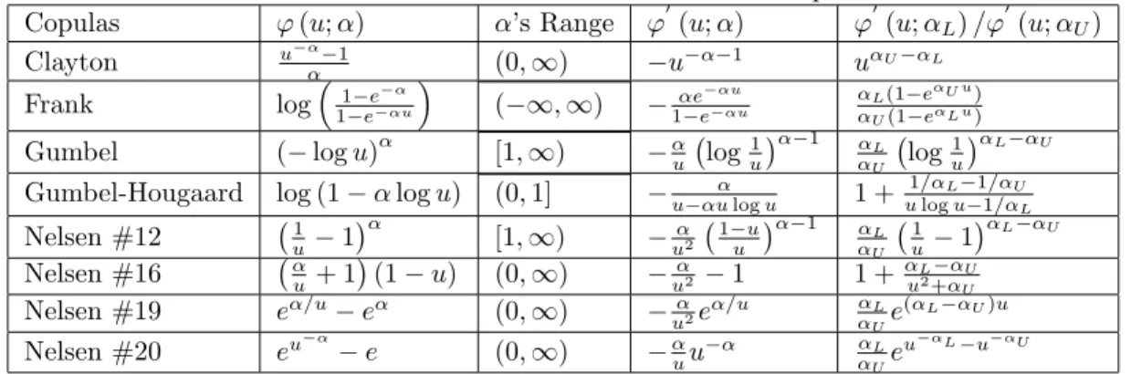
context of competing risks, Bond and Shaw (2006) have studied the so-called covariate-time transformation model in which the modelling assumption directly implies the copula invariance. Bond and Shaw (2006) show that classical competing risks models including the accelerated failure-time model and the proportional hazard model fall into their framework, see also Clayton and Cuzick (1985), Heckman and Honore (1989). Assumption (O-P-I) (ii) restricts the class of copula functions to be in a given parametric class. Informal sensitivity analysis in Zheng and Klein (1995), Huang and Zhang (2008), and Chen (2010) suggest that the bias of estimates of the marginal survival function ofY is negligible when the parametric copula misspeci…es the true copula as long as the dependence range (such as Kendall’s tau) is correctly speci…ed. This is also con…rmed in our numerical analysis in Example 2.9 below. Many one-parameter families of Archimedean copulas including Frank or Clayton copulas satisfy Assumption (O-P-I) (iii). They are either positively ordered (increasing in concordance order as the parameter increases) or negatively ordered (decreasing in concordance order as the parameter increases), see Joe (1997), Nelsen (2006), and Rivest and Wells (2001). In Table 1 below, we list a number of one-parameter families5 _{of Archimedean copulas that are ordered and}

satisfy Assumption (O-P-I) (iii).

Table 1: One-Parameter Archimedean Copulas

Copulas '(u; ) ’s Range '0(u; ) '0(u; L)=' 0 (u; U) Clayton u 1 (0;₁) u 1 _u U L Frank log ₁1 _ee u ( 1;1) e u 1 e u L(1 e U u) U(1 e L u)

Gumbel ( logu) [1;₁) _u log1_u 1 L U log

1

u

L U

Gumbel-Hougaard log (1 logu) (0;1] _{u ulogu} 1 + 1= L 1= U

ulogu 1= L Nelsen #12 1 u 1 [1;1) u2 1_uu 1 _L U 1 u 1 L U Nelsen #16 _u+ 1 (1 u) (0;₁) _u2 1 1 + _uL2_{+ U}U Nelsen #19 e =u _{e (0;1)} u2e =u L Ue ( L U)u Nelsen #20 eu _{e (0;1)} uu LUe u L _u U

Under Assumption (O-P-I), the class of generator functions is given by

x=f'x:'x( ) ='( ; ) for some 2 Ag;

where the functional form of'( ; )is known. So for a given family of ordered parametric copulas, the choice of xis equivalent to the choice ofA [ L; U]. Users could specify L; U re‡ecting their prior knowledge

on the possible dependence range giving rise to_CxL andCxU. In a sensitivity analysis, users could take L

corresponding to the independence copula and specify several values for U re‡ecting di¤erent strengths of

dependence betweenY andC; the larger U is, the larger is the deviation of the true censoring mechanism

from independence censoring. Under Assumption (O-P-I), the following equality holds:

( ) = 1 + 4

Z 1

0

'(u; )

'0_{(u; )}du: (2.16)

5_{Some of the copulas in Table 1 do not have names (or not widely known among researchers), we simply attribute them as} Nelsen’s #, as those are found by Table 4.1 appearing in Chapter 4, Nelsen (2006).

It is evident from (2.16) that perturbation on could be performed on the copula’s natural parameter . For Clayton and Gumbel copulas, it is known that Kendall’s = ₊₂ and 1 respectively, so = 0for Clayton copula and = 1 for Gumbel copula correspond to independent censoring and as increases the censoring mechanism deviates more from independent censoring. Assumption (SC) is a separation condition. It excludes cases where our copula lower bound SY (jx; U)is identical to Peterson’s lower bound SV (jx)

for allx_{2 J}.

Under Assumption (O-P-I), for'_x2 x,FY (yjx;'x)depends on'xonly through . So we denote it as

FY(yjx; )in the rest of this paper.

Proposition 2.8 Suppose Assumptions (AC), (SY), and (O-P-I) hold for allx_{2 J}. Then (i) the identi…ed set for _o is

BIO=f 2 B:FY (x0 jx; ) =qfor allx2 J and some 2 Ag; (2.17)

(ii) if Assumption (SC) holds as well, then given any in _BO

I, there is a unique ( )such that

FY(x0 jx; ( )) =q for allx2 J: (2.18)

Proof. (i) is obvious. Now given (i), it su¢ ces to show for any 1, 2 2 A (w.l.o.g we take 1 < 2),

FY(x00 jx0; 1)< FY (x00 jx0; 2)holds for the particularx0 in the separation assumption (SC). From the

conclusion in Proposition 2.3 we know thatSY(jx0; 2) SY (jx0; U) > SV(jx0)holds in terms of the

invariant generator and at locationx0. The proof follows almost verbatim from the proof of Prop. 2.3. After

equation (2.9) we shall proceed with those strict inequalities:

'0_fSY (vjx0; 2) ; 1g '0 fSY (vjx0; 2) ; 2g >' 0 fSV (vjx0) ; 1g '0 fSV (vjx0) ; 2g ; withv₂(ylx0; yux0)

for 1< 2 by (2.15) . Similar manipulation leads to'fSY yjx0; ' 2 ; 1g> 'fSY yjx0; ' 1 ; 1g, and

the copula generator is strictly decreasing, thusFY (yjx0; 1)< FY (yjx0; 2). Therefore given any in BIO

whenFY(x0 jx; ( )) =q2(0;1), we could only have a unique ( )forx2 J.

Example 2.9 (Gumbel Copula) Suppose Assumption (O-P-I) (i) and (ii) hold with the family of Gumbel copulas so

'(u; ) = ( logu) ; ₂[1;₁):

Let odenote the true value of the copula parameter. Suppose the true conditional marginal survival functions

are SY ojX(yjx) =e y=x and SCjX(cjx) =e c=x fory 0, c 0, andx >0. It is easy to show that the

conditional survival and sub-survival functions of the observable V are given by:

SV (vjx) = exp h 21= ov x i and SV;D=1(vjx) = 1 2exp h 21= ov x i ; x >0:

Suppose we know that o 2 [ L; U] or equivalently o 2 [ L; U] = h L 1 L ; U 1 U i (see Example 5.4 in Nelson, 2006). For any ₂[ L; U], (2.7) implies that fory >0;

SY (yjx; ) = exp h 21= o 1= y x i (2.19)

yielding the boundsSY(yjx; L)andSY (yjx; U)for the true survival functionSY o(yjx).

Let x= 1, o= 2 ( o= 0:5), and L = 1; U = 5 ( 2[0;0:8]). In Figure 1, we plot the true survival

function SY o(yj1) (black solid curve), our copula bounds SY (yj1; L) and SY (yj1; U) (two blue curves),

and the worst-case Peterson bounds (two red curves):

SV (yj1) = exp 21= oy and SV;D=1(yj1) +SV;D=0(0j1) = 1 2exp 2 1= o_{y +}1 2:

Some observations follow immediately. First the Peterson’s upper bound has some unpleasant feature, namely it is only pointwise sharp not functionally sharp. The upper bound on the survival function is not a proper survival function itself, more speci…cally, limy!1[SV;D=1(yj1) +SV;D=0(0j1)] = Pr (D= 0j1), which is

strictly bigger than0in nontrivial cases (see Crowder 1991; Bedford and Meilijson 1997). Second, Peterson’s bounds can be tightened signi…cantly when prior knowledge on the censoring mechanism is available. Finally, the deviation from the independent censoring assumption may not be negligible, making the sensitivity analysis necessary.

Next we illustrate the e¤ ect of misspeci…cation in the generator function (while …xing the dependence range) on the copula bounds. So instead of the Gumbel copula, we use the Clayton copula:

e

'(u;e) = u

e ₁

in (2.7) leading to SY (yjx;e) = 1 21= o h exp h 21= o_ey x i 1 i + 1 1=e : (2.20)

Example 5.4 in Nelson (2006) shows that for the Clayton copula, = _e+2e . The range for Kendall’s varying in[0;0:8]would translate to e2[0;8]. In Figure 2 we again plot the true survival functionSY o(yj1) (black

solid curve) and the copula boundsSY (yj1; L)andSY (yj1; U)(two blue curves) using the correctly speci…ed

Gumbel copula. In addition, we also plot the misspeci…ed copula bounds SY (yj1;eL) andSY (yj1;eU)(the

two red curves) computed using the Clayton copula, where eL = 0and eU = 8. Notice that the two sets of

copula bounds are almost identical. This observation is consistent with existing simulation results showing the negligible bias in the estimated bounds with misspeci…ed copula function as long as the dependence range is correctly speci…ed, see Zheng and Klein (1995), Huang and Zhang (2008), and Chen (2010).

Finally we complete this example by deriving the identi…ed set for _o. By the restriction thatSY( ojx; ) =

1 q, we get: o2 log 1 1 q 2 1= U 1= o_;log 1 1 q 2 1= L 1= o _{: (2.21)}

In terms of the corresponding[ L; U], we get

o2 log 1 1 q 2 1 U 1= o_;log 1 1 q 2 1 L 1= o _:

In this example, the quantile regression coe¢ cient is interval identi…ed (Manski, 2003) and there is one-to-one correspondence between the quantile regression coe¢ cient and the dependence level characterized by Kendall’s tau.

It is obvious from the expression for SY (yjx; )in (2.19) that Assumption (SC) holds for all x >0 and

all …nite U.

3

Asymptotic Con…dence Sets for

In the rest of this paper, we suppose Assumptions (AC), (SY), and (O-P-I) hold for all x _{2 J}. In this section, we construct two asymptotic con…dence sets for _o based on the identi…ed set_BO

I in (2.17):

BOI =f 2 B:FY (x0 jx; ) =qfor allx2 J and some 2 Ag:

The identi…ed set_BO_I allowsX to be any random variable, discrete or continuous or mixed. In what follows, we work explicitly with mixed type regressors, so X Xc; Xd with both continuous component Xc =

Xc

1; Xpc and discrete componentXd= X1d; Xrd . Furthermore,Xjd takes the values0;1; :::; cj 1for

j= 1; :::; r.

De…ne the population criterion function as

T( ) = min 2[ L; U] T( ; ) = min 2[ L; U] Z J [FY (x0 jx; ) q] 2 f_X2 (x)dx, (3.1)

where_J =_Jc _J1d ::: _Jrd, with_Jc int(_Xc)being compact and_Jjd =_f0;1; :::; cjgforj = 1; :::; r. Also

the integralRdxis understood to beP_xd R

d (xc), integrating over the counting measure on_J1d ::: Jrd

and Lebesgue measure on_Xc_{. Our CSs are based on the sample version ofT( ; )de…ned as:}

Tn( ; ) = Z J h b F(x0 _jx; ) qi2fb_X2 (x)dx; (3.2) whereFb(_jx; ) is the plug-in estimator ofFY (jx; )introduced in the subsection below andfbX(x)is the

kernel-type density estimator offX(x)de…ned below:

b fX(x) = 1 n n X i=1 W (x; Xi) (3.3) where W (x; Xi) = Kh(xc Xic)L xd; Xid; , = (h; ) = (h; 1; ; r), Kh( ) = h pK(=h) denotes

the standard kernel function for continuous regressors,6 _{whereasL(; ; )is the Aitchison and Aitken (1976)}

kernel: L xd; X_id; = r Y j=1 ( j=(cj 1))Nij(x)(1 j)1 Nij(x)

with Nij(x) = I Xijd 6=xdj for j = 1; :::; r. For the advantage of smoothing discrete regressors over the

standard frequency approach, see Hall, Racine and Li (2004), Li and Racine (2007). We propose two test statistics from which we could draw inference on _o:

b Tn( ) =Tn( ;b( )) and (3.4) e Tn( ) =Tn( ;e( )); (3.5) where b( ) ₂ arg min 2[ L; U] Tn( ; ) and e( ) ₂ arg min 2[ L; U] Tn( ; ) Bbn( ; ) q b( ; )

withBbn( ; )and b( ; )being uniformly consistent estimators ofBn( ; ) and ( ; )de…ned in (B.6)

(B.8) in Appendix B. Our CSs for _o with asymptotic level(1 )are de…ned as

CSN 1 ;Tbn= 8 < : 2 B: nhp=2 _Tb n( ) Bbn( ;b( )) q b( ;b( )) z1 =2 9 = ; and (3.6) CSN_{1 ;Te} n = 8 < : 2 B: nhp=2 _Te n( ) Bbn( ;e( )) q b( ;e( )) z1 =2 9 = ;; (3.7)

wherez1 =2is the(1 =2)-th percentile of the standard normal distribution.

6_{In typical applications, discrete regressors would have di¤erent support and cardinality, so we let change withr; for} notational brevity we use single bandwidth for all continuous regressors.

We show in the next section that under conditions including Assumption (O-P-I) and the conditions of Proposition 2.6, bothCSN

1 ;Tbn andCS

N

1 ;Ten are asymptotically valid and non-conservative CSs for o.

By varying L and U, both CSs can be used to check sensitivity of inference for o to the independent

censoring assumption. In contrast to most CSs for partially identi…ed parameters, the CSs CSN

1 ;Tbn and

CSN

1 ;Ten are straightforward to implement. This is especially important in the context of a sensitivity

analysis since they are typically computed several times for di¤erent ranges of the copula parameter .

Remark 3.1 For a given _{2 BI}O, the test statistics Tbn( )and Ten( )in (3.4) and (3.5) resemble the test

statistics for consistent model speci…cation testing based on kernel estimators, see Fan (1994), Fan and Li (1996), and Zheng (1996) and many subsequent works in the literature.7 _{Indeed, as in these papers, we show}

later that under suitable conditions including the separation assumption (SC), the asymptotic distributions of

b

Tn( )andTen( )are normal justifying the CSsCS₁N _;Tb

n andCS

N

1 ;Ten de…ned in (3.6) and (3.7). Thus the

CSs CSN

1 ;Tbn andCS

N

1 ;Ten for o are intrinsically linked to speci…cation tests for the class of parametric

copulas with generator function' , _{2 A}.

Remark 3.2 An alternative approach to construcing CS for _o is to make use of the inequality constraints on _o in Proposition 2.6: FL(x0 ojx) q FU(x0 ojx)for all x2 J. For instance, one could adopt the

following criterion function:

Z J h b F(x0 _jx; L) q i2 _ b f_X2 (x)dx+ Z J h b F(x0 _jx; U) q i2 + b f_X2 (x)dx: (3.8)

Compared with Tbn( ) or Ten( ), this approach su¤ ers from several drawbacks. First, the asymptotic

dis-tribution of the statistic in (3.8) is di¢ cult to establish; Second, similar to existing work on inference for parameters de…ned by moment inequalities such as Andrews and Shi (2013), variants of the ‘generalized mo-ment selection’may be needed introducing additional parameters that practitioners have to select. In contrast, CSs based onTbn( )or Ten( )circumvent this because they rely on equality constraints only; Third, let

BO=f 2 B:FL(x0 ojx) q FU(x0 ojx) for allx2 J g:

Proposition 2.6 only shows that_BO is an outer set of the identi…ed setBOI , i.e.,BIO BO, but it is not clear

whether _BO BIO.

3.1

The Plug-in Estimator of

F

(

y

j

x

; )

Our test statistics depend on an estimator of FY (x0 jx; ) or generally of FY (yjx; ) de…ned in (2.7).

Throughout this section we will suppress the subscript Y in its conditional distribution or survival func-tions unless otherwise emphasized. When the censoring mechanism is independent conditional on covariates, Dabrowska (1987, 1989) studies the consistency and weak convergence of the so-called conditional Kaplan-Meier estimator originally proposed by Beran in an unpublished report. Under dependent censoring mech-anism, Braekers and Veraverbeke (2005) generalize the copula-graphic methods in Rivest and Wells (2001) 7_{Similar speci…cation testing procedures with mixed type regressors could be found in Fan, Li and Min (2006) and Hsiao,} Li and Racine (2007).

to the case where X is univariate and non-stochastic. In this section we propose a plug-in estimator of

FY(yjx; )using its expression in (2.7).

We …rst introduce the Nadaraya-Watson kernel estimators ofFV;D=1(vjx)andFV (vjx):

b FV;D=1(vjx) = n X i=1 wn (x; Xi)I[Vi v; Di= 1] and b FV (vjx) = n X i=1 wn (x; Xi)I[Vi v]; wherewn (x; Xi) =W (x; Xi)= Pn

j=1W (x; Xj), withW (; )de…ned in the previous subsection. In view

of our Lemma 2.1, it is natural to work with the plug-in type estimator for the conditional distribution functions indexed by : b F(y_jx; ) = 1 ' 1 Z y ylx '0 n b SV (sjx) ; o dFbV;D=1(sjx) ; (3.9) = 1 ' 1 2 4 X Vi y;Di=1 '0 SbV (Vijx) ; wn (x; Xi) ; 3 5:

Remark 3.3 An alternative estimator ofFY (yjx; )is the copula graphic estimator introduced in Braekers

and Veraverbeke (2005) denoted asFe(y_jx; ) = 1 Se(y_jx; ), where

e S(y_jx; ) (3.10) = =' 1 8 < : X Vi y;Di=1 h ' SbV Vi jx ; ' SbV Vi jx wn (x; Xi) ; i ; 9 = ;:

The estimator Fe(y_jx; ) generalizes the conditional kernel Kaplan-Meier estimator proposed in Dabrowska (1987, 1989) to allow for conditional dependent censoring characterized by the generator function '( ; ). When'(t; ) = log (1=t),(Y; C)are independent conditional on X=xandFe(y_jx; ) reduces to the condi-tional kernel Kaplan-Meier estimator in Dabrowska (1987, 1989),

e FInd(yjx) = 1 2 4 Y V(i) y 1 wn x; X[i] 1 Pi_j=11wn x; X[j] !D[i]3 5 (3.11) where V(i) n

i=1denote the order statistics and D[i]; X[i]

n

i=1denote the induced order statistics of the sample.

The above estimator resembles the traditional Kaplan-Meier estimator closely, replacing the empirical weight

n 1_{with the kernel weightw}

n (x; Xi). As shown in Lemma A.3, the two estimatorsFb(yjx; )andFe(yjx; )

are …rst order asymptotically equivalent.

4

Asymptotic Validity and Bootstrap Con…dence Sets

In this section, we …rst establish a uniform asymptotic linear representation of the plug-in estimator of

FY(yjx; ), then establish asymptotic validity of the CSs CS₁N _;Tb

n and CS

N

1 ;Ten, and lastly construct

4.1

Asymptotic Linear Representation of

F

b

(

y

j

x;

)

We …rst present regularity assumptions used to establish the asymptotic linear representation ofFb(y_jx; ). The random vector Zi = (Vi; Di; Xi) stacks all the observable random variables. To ease the notational

burden, we assume that the support of the conditional distribution function ofY is …xed at[yl; yu], invariant

with respect tox. In addition, we let' (u) ='(u; )throughout the rest of this paper and let

_ '0 (u) @ @ ' 0 _{(u) and'_} 1_(u) @ @ ' 1_(u):

Assumption (D).(i) The random variableXc _{has an absolutely continuous and bounded density w.r.t}

the Lebsegue measure in_Rp_{, andinf}

x2J fX(x)>0 for the compact subsetJ in (3.1); (ii) The marginal

density function fX(x) = fX xc; xd satis…es 8xd, xc !fX xc; xd is s-order continuously di¤erentiable

over the set_Jc _{and thes-order derivatives are bounded; (iii) There existsy}0

uin the support ofY and 0>0

such that

SV y0ujx 0 a.s. x2 J: (3.12) Assumption (F). (i) The two conditional sub-distribution functions have continuous bounded condi-tional sub-density functionsfV;D=j(vjx),j = 0;1uniformly forx2 J; (ii) Along thexc-axis the conditional

sub distribution functions satisfy:

8v₂ yl; y0u and 8xd, xc !FV;D=1 vjxc; xd ; x!FV;D=0 vjxc; xd are s-order continuously

di¤eren-tiable over the set_Jc_{, with boundeds-order derivatives.}

Assumption (G). (i) Along theu-axis, the generator function' ( )is third order continuously di¤er-entiable with'(3)( ) 0 and'(3)( )remains bounded uniformly for_{8 2 A} and for₈u₂[ 0;1]. Moreover

'0 ( )is bounded away from0 uniformly for _{2 A}and u₂[ 0;1]for the 0 de…ned in (3.12);

(ii) The Lipschitz continuity property with respect to holds for ( ) = 1='0 ( )or ( ) ='00( )with positive constantL:

sup

u2[ 0;1]

1(u) 2(u) Lj 1 2j:

Assumption (H). (i) The bandwidth satis…es the following conditions: h_! 0,_lognhp_{n ! 1}, nh2s _!0, nh2s+p

logn !0 and

(logn)2

nh3p=2 !0asn! 1;

(ii) For all j= 1; ; r, j!0 and nhp 2j

logn !0, asn! 1.

Assumption (K). Let K(u) = Qp_j=1k(uj), where k( ) is a bounded s-order kernel function with

compact support, i.e.,

Z

k(u)du= 1and

Z

ujk(u)du= 0forj= 1; :::; s 1.

Moreover it can be written as (p(x)), with ( )being of bounded variation and p(x)a real polynomial on_R.

Assumptions (D)(i), (ii) and (F) are standard assumptions used to establish asymptotic properties of estimators or test statistics that are functionals of kernel type regression estimators (see Li and Racine,

2007). Assumption (D)(iii) plays a similar role to Assumption (D)(i), because most generator functions have unbounded derivatives at0, see Table 1. Assumption (D)(iii) allows us to avoid having to deal with such explosive behavior of the generator function and require Assumption (G) (i) only when establishing the linear representation ofFb(y_jx; ), see the expression in (3.9).8 _{It can be relaxed by imposing suitable}

restrictions on the tail behavior of the generator function at the expense of more tedious proofs. Apropos of the requirement on the copula generator, the di¤erentiability and non-vanishing …rst order derivative are almost necessary in view of the following uniform asymptotic linear representation. The Lipschitz continuity in Assumption (G)(ii) is used to prove uniformity of the linear representation over and it also simpli…es the convergence argument for b( )or e( )when we apply the local U-process machinery. The condition on the bandwidth is standard in kernel estimation problem, and we undersmooth a bit to kill the bias term, facilitating the inference procedure. Under Assumption (K), we have the following VC-type functional class due to Nolan and Pollard (1987):

K= K h 1(x ) :x_{2 R}p,h >0 :

An explicit construction ofk( )satisfying the above requirement could be found in Section 1.2.2 in Tsybakov (2008) based on Legendre polynomials.

Theorem 4.1 Under Assumptions (D)-(K), it holds that

b F(y_jx; ) FY (yjx; ) = 1 nfX(x) n X i=1 W (x; Xi)g(yjZi; x; ) +Rn(y; x; ); (3.13) whereg(y_jZi; x; ) =c(yjZi; x; ) +b(yjZi; x; ) in which c(y_jZi; x; ) = 1 '0 _{fSY(yjx; )g}[ Z y yl '00_fSV (vjx)g[I(Vi v) FV(vjXi)]dFV;D=1(vjx) (3.14) '0 _fSV (yjx)g[I(Vi v; Di= 1) FV;D=1(yjXi)] Z y yl '00_fSV (vjx)g[I(Vi v; Di= 1) FV;D=1(vjXi)]dFV (vjx)]; b(y_jZi; x; ) = 1 '0 _{fSY (yjx; )g}[ Z y yl '00_fSV (vjx)g[FV (vjXi) FV (vjx)]dFV;D=1(vjx) (3.15) '0 _fSV (yjx)g[FV;D=1(yjXi) FV;D=1(yjx)] Z y yl '00_fSV (vjx)g[FV;D=1(yjXi) FV;D=1(vjx)]dFV (vjx)]

andRn(y; x; )satis…es that

sup 2A sup x2J sup y2[yl;yu0] jRn(y; x; )j=Op logn nhp :

8_{At the right end point1, only Gumbel copula generator has'}0_{(1) = 0in our Table 1, one could simply modify the above} requirement fort2[ 0; 1], with some approporiate 1<1.

Compared with the result for the copula-graphic estimatorFe(y_jx; )in Braekers and Veraverbeke (2005), (3.13) holds uniformly forx _{2 J X} with a better rate for the remainder term, where the density of X

stays away from 0 on _J, and our covariate is a multivariate random variable rather than univariate …xed design.

Remark 4.2 HoldingX =x…xed and' …xed at some _{2 A}, we could also establish the weak convergence of the conditional empirical process: npnhph_Fb_{(yjx; ) F}

Y (yjx; )

i

:y₂ yl; yu0

o

. It can be shown that the process is stochastically equicontinuous w.r.t. certain pseudo metric. We refer the readers to Braekers and Veraverbeke (2005) for a detailed proof for the copula-graphic estimatorFe(y_jx; ).

We can also establish the uniform consistency of Fb(y_jx; ), which we record as a corollary below. Its proof is actually shown in Lemma A.3 when characterizing the order ofRn3(y; x; )de…ned in Appendix A.

Corollary 4.3 Under the Assumptions (D)-(K), it holds that

sup 2A sup x2J sup y2[yl;y0u] jFb(y_jx; ) FY (yjx; )j=Op r logn nhp ! :

In particular, it holds if we sety=x0 for those x0 ₂ yl; y0u .

4.2

Validity of the Asymptotic Con…dence Sets

In order to prove the asymptotic exactness of the con…dence sets de…ned in (3.6) and (3.7), we show that

b

Tn( ) and Ten( )are both asymptotically normal upon proper centering and normalization. Noting that

those two statistics resemble the population criterion function closely, we show below that b( )and e( )

converge in probability to ( )and prove the stochastic equicontinuity (SE) of[Tn( ; ) Bn( ; )]w.r.t

in the local neighborhood of ( )whose radius is determined by the convergence rate of b( )or e( )

to ( ). Proving consistency and getting convergence rate for estimators obtained from minimizing a kernel based criterion function is akin to a problem from smooth minimum distance estimation, as shown in Linton (1997, 1998), also see Lavergne and Patilea (2013) on a recent account. For = ( ), the asymptotic distribution of[Tn( ; ) Bn( ; )]is determined by a degenerateU-statistic similar to the test

statistics in Hardle and Mammen (1993), Fan (1994), Fan and Li (1996), and Zheng (1996); when ₆= ( ),

[Tn( ; ) Bn( ; )]could be decomposed as the degenerate U-statistic, a non-degenerate U-statistic and

the deterministic drifting term: R

J[FY (x0 jx; ) q]

2

f2

X(x)dx. The SE of [Tn( ; ) Bn( ; )] would

be proved by showing the SE of the degenerate U-process and negligibility of the other two terms when approaches ( )su¢ ciently fast.

We need two more sets of assumptions to show the validity of our con…dence sets, one (Assumptions (V0) and (V1)) forCSN

1 ;Tbn and one (Assumptions (V0) and (V2)) forCS

N

1 ;Ten. Assumption (V0). For all _{2 B}, x0 ₂ yl; yu0 for allx2 J.

Assumption (V1). (i) For any _{2 B}O_I, the corresponding ( ) belongs to the interior of_A; (ii) In addition to Assumption (H), we assume thatnh2s_!0; (iii) In addition to Assumption (G), those functions

_

'0 (u),'_ 1(u)exist and are continuous and bounded in the range of[ 0;1]and[0;1)respectively. Assumption (V2). (i) In addition to Assumption (H), there exists a sequence"n!0such that

q

n

logn"n!

1andnhp_"

n!0; (ii) In addition to Assumption (G), the Lipschitz continuity property with respect to

holds for ( ) = 1='0 ( )or ( ) ='00( )with positive constantLfrom below:

L_j 1 2j sup

u2[ 0;1]

1(u) 2(u) :

Assumption (V0) is used for both CSs. It ensures that all the conditional quantiles of potential interest stay su¢ ciently far away from the right end support point ofV. When independent censoring is assumed, similar restrictions have also appeared in Peng and Huang (2008), Wang and Wang (2009) for in a neigh-borhood of the (point identi…ed) true _o. There is a distinction between Assumption (V1) and Assumption (V2) because of the slightly di¤erent arguments used in the proofs for CSN

1 ;Tbn andCS

N

1 ;Ten. The

con-sistency of b( ) follows the standard way to contrast sample criterion function and population criterion function, viewed as a minimum distance estimator. Its rate of convergence is shown once the requirement that ( )stays in the interior and enough smoothness (w.r.t ) on the generator function are satis…ed. In comparison, a di¤erent route is taken for e( )as in Santos (2006). Its consistency and rate of convergence will be achieved through the di¤erent convergence stochastic orders of the test statistic and a careful study of the local neighborhood of the ’null’set for (see Santos, 2006):

A"n

o = 2 A:

Z J

[FY (x0 jx; ) q]2fX2 (x)dx "n; with"n!0 : (3.16)

Notice that when "n !0, A"on will shrink to the singleton f ( )g; on the other hand, when 2 A= "on, the

sample criterion function would be shown to be explosive.

The …rst main result in this section establishes the asymptotic distributions of the test statistics Tbn( )

andTen( )for 2 BIO, thereafter the asymptotic size property of our con…dence sets follows immediately.

Proposition 4.4 Suppose Assumptions (SC), (D)-(K), and (V0) hold, then for _{2 B}O

I with the unique

( ),

nhp=2[Tn( ; ( )) Bn( ; ( ))]

p

( ; ( )) =)N(0;1): (3.17)

In addition if (V1) holds, we have:

nhp=2 h Tn( ;b( )) Bbn( ;b( )) i q b( ;b( )) =₎N(0;1) ; (3.18) if (V2) holds, we have: nhp=2h_T n( ;e( )) Bbn( ;e( )) i q b( ;e( )) =₎N(0;1); (3.19)

where Bn( ; ) =n 1h p

R

K2(u)duR 2(x0 _jx; )fX(x)dx in which 2(x0 jx; ) is de…ned in (C.2) in

Appendix C, and ( ; ) is de…ned in (B.8) in Appendix B with uniformly consistent estimators Bbn( ; )

and b( ; ) respectively.

Theorem 4.5 Under the assumptions (SC), (D)-(K), and (V0), our con…dence sets have pointwisely as-ymptotic exact size: for _{8 2 B}O

I , if (V1) holds, we get: limn!1Pr n

2CSN

1 ;Tbn o

= 1 ; or if (V2) holds, we get: limn!1Pr

n

2CSN

1 ;Ten o

= 1 :

Remark 4.6 Both test statistics and con…dence sets have their own merits. Tbn( )circumvents the need to

estimate the complicated drifting term and asymptotic variance term when the minimization over _{2 A}is conducted; on the other hand, even without the separation assumption (SC), the procedure based on Ten( )

is still asymptotically valid although may be conservative, similar to Jun and Pinske (2009) in a di¤ erent context: lim sup n Pr 8 < :min2A nhp=2 h Tn( ; ) Bbn( ; ) i q b( ; ( )) z1 =2 9 = ; lim n Pr 8 < : nhp=2h_T n( ; ( )) Bbn( ; ( )) i q b( ; ( )) z1 =2 9 = ; = 1 :

4.3

Bootstrap Con…dence Sets

It is well documented in the literature on model speci…cation testing that the normal approximation of the distribution of the kernel-based test statistics may not work well in small samples, see Hardle and Mammen (1993) and resampling methods such as bootstrap may be used. Below we present bootstrap analogues of the asymptotic con…dence setsCSN

1 ;Tbn andCS N 1 ;Ten. Let T_n;b( ; ) Z J " 1 n n X i=1 W (x; Xi)cb x 0 jZi; x; #2 dx; where c_b(y_jZi; x; ) (3.20) = Mi;b '0 n_Sb_{(yjx; )}o[ Z y yl '00nSbV (vjx) o h I(Vi v) FbV (vjXi) i dFbV;D=1(vjx) '0 n b SV (yjx) o h I(Vi v; Di= 1) FbV;D=1(yjXi) i Z y yl '00nSbV (vjx) o h I(Vi v; Di= 1) FbV;D=1(vjXi) i dFbV (vjx)]

in which the perturbation variablesnM_i;bon

i=1are independently generated with zero mean and unit variance

we de…neT_n;b( ;b( ))andT_n;b( ;e( ))accordingly.9 We could generate nM_i;bon

i=1 for b = 1; :::; B and obtain

n T_n;b( ;b( ))oB b=1 or n T_n;b( ;e( ))oB b=1.

The bootstrap critical values are de…ned as

cB_n;Tb n( ;1 ) = inf ( t: 1 B B X b=1 I n nhp=2T_n;b( ;b( )) t o 1 ) and cB_n;Te n( ;1 ) = inf ( t: 1 B B X b=1 I n nhp=2T_n;b( ;e( )) t o 1 ) :

Hence the following two bootstrap con…dence sets are immediate:

CSB 1 ;Tbn = n 2 B:nhp=2Tbn( ) cB_n;Tb n( ;1 ) o and CSB 1 ;Ten = n 2 B:nhp=2Ten( ) cB_n;Te n( ;1 ) o :

Theorem 4.7 Under the assumptions (AC), (D)-(K), and (V0), our bootstrap con…dence sets have point-wisely asymptotic exact size: for_{8 2 BI}O, if (V1) holds, we get: limn!1Pr

n

2CSB

1 ;Tbn o

= 1 ; or if (V2) holds, we get: limn!1Pr

n 2CSB 1 ;Ten o = 1 :

5

An Empirical Application

In this section, we illustrate our methodology on a real data set used in Wang and Wang (2009). The data comes from a study on the survival of patients after acute myocardial infarction conducted at the University Clinical Center in Ljubljana and is publicly available in R packagerelsurv. It consists ofn= 1;040

observations with493 censored observations. The variable of interest, i.e., the survival time, is recorded in days and we transform it into the unit scale[0;1]by the empirical probability integral transformation. There are two regressors of mixed type; the discrete regressor is Gender (with 751 observations from Male vs. 289 observations from Female) and the continuous regressor is Age (we again transform the original data into the unit scale between [0;1]).10 _{The exact cause of censoring is unknown in this data, however in typical}

clinical studies censoring is not merely of administrative type (censoring occurs because the study simply terminates). Patients might be removed if there is evidence that treatment is ine¤ective, or patients withdraw themselves because of side e¤ects or they die due to other causes (Fleming and Harrington, 1991). Hence it is reasonable to expect some positive dependence betweenY andC in those situations.

We compare our con…dence set CSB

95%;Tbn with two bootstrap con…dence intervals in Portnoy (2003),

Peng and Huang (2008) (Por, PH in Table 2 below respectively) where conditional independent censoring is assumed. Those two approaches could be automatically implemented in Roger Koenker’s R package

quantreg. Linear quantile regressions, with intercept and slope , are …tted on subsets splitted according 9_{One could bootstrap the drifting term when calculatingTe}

n( )

1 0_{In comparison, Wang and Wang (2009) take the log transform of the original survival time. Also, even though the procedure} in Wang and Wang (2009) calls for ordinary kernel smoothing across the variable Age, they still work with the original one, which is integer-valued.

to gender groups and we report the bootstrap con…dence intervals on the slope coe¢ cient . Notice that the data between di¤erent gender groups are very unbalanced, which justi…es the smoothing across the discrete regressor here (Li and Racine, 2007). Referring to the actual implementation of our approach, since the continuous regressor is univariate, we letK(u) = 15

16 1 u

2 2_{, the bisquare kernel which is a second order}

kernel. Moreover the two tuning parameters are set to be h= 2n 1=4_{, = n} 1=2_{, and the truncation of}

the integral is restricted to be_J = [0:1;0:9]. Also the perturbation variableM_i;bin the bootstrap weight is taken to be standard normal. Needless to say, our procedure is computationally more intensive as for every regression coe¢ cient under consideration, a minimization over is carried out and bootstrap is needed to obtain the critical value. To reduce computational cost, we simply set the the number of bootstrap replications at 100 and do a grid search over ₂ [ 5;1] with grid length equal to0:01. Notice that our construction of con…dence set leads to simultaneous inference on both the slope and the intercept . However, the bootstrap intervals in Portnoy (2003), Peng and Huang (2008) are for the slope and intercept separately. For fair comparison, we have picked a projection based version of ours by considering all not rejected while runs over in[0;1]with a grid length0:01.11 _{To check the sensitivity of conclusions from}

maintaining ICM assumption, we consider two scenarios, small vs. moderate deviations. In the former case, we set ₂[0;0:2]whereas in the latter case ₂[0;0:5]. Both con…dence sets based on Clayton copula and Gumbel copula are reported to examine the e¤ect of employing di¤erent copula generator functions when the speci…ed dependence level coincides. The results are reported in Table 2 below, where DCM denotes dependent censoring mechanism.

Some remarks follow from Table 2. First of all, our con…dence sets turn out to be intervals for this particular case, so there are no holes in between. Second, despite we choose the projection based inference (which might be conservative) and allow for a wider range of dependence, our con…dence intervals are not necessarily wider than those inPor, PH for the female group. The frequency approach by splitting the data leaves too few observations in the female group and as noted in Wang and Wang (2009), Por, PH tend to be unstable for small samples. Third, the conclusion on negative e¤ect (the sign) of aging on the survival time is robust even when we allow for ₂[0;0:5], but the one on the exact magnitude might change. For example, in the male group when q= 3=4, the ICM intervals lead to the accelerating e¤ect (_{j j}>1) from aging, but this could be overturned when we allow for moderate positive dependence. Finally, the di¤erence between …tting a Clayton and Gumbel is almost negligible, never larger than 0:08. So the exact shape of a generator function plays only a minor role.

6

Concluding Remarks

Assuming an Archimedean copula for the dependent variableY and the censoring variableC, we have pro-posed a two-step method for studying partial identi…cation of the quantile coe¢ cient _oin quantile regression 1 1_{The reason we set the parameter spaceBto be [0;1] [ 5;1]is that it includes the widest interval coming from Portnoy} (2003), Peng and Huang (2008) and is slightly enlarged.

Table 2: Con…dence Sets Male Female q 1=4 1=2 3=4 1=4 1=2