Modelling water quality, bioindication and population
dynamics in lotic ecosystems using neural networks
Ingrid M. Schleiter
a,*, Dietrich Borchardt
a, Ru¨diger Wagner
c,
Thomas Dapper
c, Klaus-Dieter Schmidt
c, Hans-Heinrich Schmidt
b,
Heinrich Werner
caDepartment of Sanitary and En6ironmental Engineering,Uni6ersity of Kassel,Kurt-Wolters-Strasse3,D-34125Kassel,Germany bLimnologische Flußstation,Max-Planck-Gesellschaft,Schlitz,Germany
cDepartment of Mathematics/Computer Science,Uni6ersity of Kassel,Kassel,Germany
Abstract
The assessment of properties and processes of running waters is a major issue in aquatic environmental management. Because system analysis and prediction with deterministic and stochastic models is often limited by the complexity and dynamic nature of these ecosystems, supplementary or alternative methods have to be developed. We tested the suitability of various types of artificial neural networks for system analysis and impact assessment in different fields: (1) temporal dynamics of water quality based on weather, urban storm-water run-off and waste-water effluents; (2) bioindication of chemical and hydromorphological properties using benthic macroinvertebrates; and (3) long-term population dynamics of aquatic insects. Specific pre-processing methods and neural models were developed to assess relations among complex variables with high levels of significance. For example, the diurnal variation of oxygen concentration (modelled from precipitation and oxygen of the preceding day;R2=0.79), population dynamics
of emerging aquatic insects (modelled from discharge, water temperature and abundance of the parental generation;
R2=0.93), and water quality and habitat characteristics as indicated by selected sensitive benthic organisms (e.g.
R2=0.83 for pH andR2=0.82 for diversity of substrate, using five out of 248 species). Our results demonstrate that
neural networks and modelling techniques can conveniently be applied to the above mentioned fields because of their specific features compared with classical methods. Particularly, they can be used to reduce the complexity of data sets by identifying important (functional) inter-relationships and key variables. Thus, complex systems can be reasonably simplified in clear models with low measuring and computing effort. This allows new insights about functional relationships of ecosystems with the potential to improve the assessment of complex impact factors and ecological predictions. © 1999 Elsevier Science B.V. All rights reserved.
Keywords:Artificial neural networks; Stream invertebrates; Population dynamics; Impact assessment; Bioindication; Time-series www.elsevier.com/locate/ecomodel
* Corresponding author. Fax: +49-561-8043642.
E-mail address:[email protected] (I.M. Schleiter)
0304-3800/99/$ - see front matter © 1999 Elsevier Science B.V. All rights reserved. PII: S 0 3 0 4 - 3 8 0 0 ( 9 9 ) 0 0 1 0 8 - 8
I.M.Schleiter et al./Ecological Modelling120 (1999) 271 – 286
272
1. Introduction
The physical and chemical properties of running waters and their effects on the community are driven by numerous environmental variables such as climatic conditions, production – respiration ra-tio, urban storm-water run-off and waste-water effluents. The underlying interactions and depen-dencies are only partially understood. Further-more, data for the calibration of theoretical models often are qualitatively or quantitatively insufficient. Because the knowledge of species – habitat interrelations remains insufficient, an inte-grative and, in consequence, prognostic assessment of ecosystem properties is not presently available (e.g. Vannote et al., 1980; Statzner et al., 1988; Townsend, 1989; Statzner et al., 1994; Townsend and Hildrew, 1994; Bayerisches Lande-samt fu¨r Wasserwirtschaft, 1998).
Ecosystem analysis and prediction with empiri-cal statistiempiri-cal and analytiempiri-cal methods are often limited by the spatially complex and temporally dynamics of ecological processes. This is one rea-son for the typically non-linear interrelations of variables and species with data being not normally distributed. Therefore, alternative mathematical methods have to be developed. Artificial neural networks (ANNs) provide an attractive alternative tool for analysing ecological data and for mod-elling due to their specific features such as non-lin-earity, adaptivity (i.e. learning from examples), generalisation and model independence (no a-pri-ori model needed).
ANNs have been applied to various fields of aquatic sciences and engineering, such as mod-elling water quality (e.g. Daniell and Wundke, 1993; Maier and Dandy, 1993, 1994, 1996a,b; Lachtermacher and Fuller, 1994; Schizas et al., 1994; Maier, 1995a; Winkler and Voigtla¨nder, 1995; Kaluli et al., 1998; Wen and Lee, 1998) and relating community characteristics with environ-mental variables (e.g. Chon et al., 1996; Lek et al., 1996; Recknagel, 1997; Recknagel et al., 1997, 1998; Gue´gan et al., 1998; Lee et al., 1998; Maier et al., 1998). Additional articles are found in this issue and in a review by Maier (1995b), focusing on the prediction of environmental, hydrological and water resources data.
In this paper we present results of the appli-cability of ANNs in the following fields: (1) dy-namics of water quality as influenced by meteorology, urban storm-water run-off and waste-water effluents; (2) bioindication of chemi-cal and hydromorphologichemi-cal habitat characteris-tics with benthic macroinvertebrates; and (3) prediction of population dynamics of aquatic insects.
The general objectives of this paper are to demonstrate the potential and limitations of ANNs and other modelling techniques for data analysis, impact assessment and ecological predic-tion in running waters, and to specify the general conditions for applications of ANNs, such as selection of relevant input variables, training con-ditions, network type and forecasting period.
2. Material and methods
We used multi-layer-perceptrons based on the Backpropagation (BP) algorithm (Rumelhart et al., 1986) and two-dimensional, motoric feature maps (FM; Ritter et al., 1994). A special variant of the BP-network type, the so-called senso-net (Dapper, 1998), was also used to determine the most important input variables (sensitivity analy-sis). Senso-nets include an additional weight for each input neuron representing the relevance (sen-sitivity) of the corresponding input parameter for the neural model. The sensitivities are adapted during the training process of the network. Appro-priate subsets of potential input variables can be selected according to these sensitivities. In contrast to most statistical methods, the dimension-reduc-ing techniques based on neural networks have the ability to map non-linear coherences (in this appli-cation, between species abundance and environ-mental variables). The neural networks and modelling techniques used for our experiments are described in Werner et al. (1999). The generalisa-tion performance, E, of the networks was calcu-lated as: E=1 2n % n i=1 %c j=1 (yij−yˆij)2 (1)
wherenis the number of samples in the test set;c is the number of output neurons; yij is the
mea-sured values; andyˆijis the modelled values.
For each variable and network type, we trained a number of networks and calculated E(minima, maxima, mean and median). We used the determi-nation coefficientR2between measured and
mod-elled data as a second standard measure of model quality. Unless otherwise specified, the results in-dicate Emin andR2max.
Prediction of water quality variables at the river Lahn (topic 1) was based on both on data from studies on a small running water body (Kuhbach (Germany); Borchardt et al., 1997) and a larger stream (Lahn at Limburg (Germany)), using dif-ferent ANNs. Basic data were daily meteorologi-cal variables (precipitation, radiation), discharge and water quality data (oxygen, conductivity, pH, water temperature) obtained above and below the waste water treatment plant of Limburg (main characteristics summarised in Table 1). Modelling daily maxima and minima was based on routine government data in 1995 (365 day-sets), whereas for modelling the diurnal fluctuation was based on data from a scientific study (150 day-sets) from April to October 1996. The data were used with-out pre-processing either as compact time inter-vals or as alternating days distributed into a training and a test data set at a ratio of 1:1, 2:1 and 3:1, respectively. Different network types
were trained with several combinations of input variables and histories of varying lengths (see Table 2).
Functional relationships between water quality, habitat characteristics and colonisation patterns of benthic macroinvertebrates (topic 2), were based on measurements of ten chemical and seven hydromorphological variables (Table 3), and the abundance of 248 species from eight small streams in Central Hesse (Germany). The experiments used the daily maxima of each variable over a one year period, except for oxygen where the mini-mum was used. The data were analysed with Pearson correlation and stepwise forward regres-sion analysis (SPSS, 1997), and sensitivity analysis on Senso-nets. The pre-processing was used to identify those species which have significant inter-relations with the variables in question, and thus may be used as bioindicators. The chemical and morphological variables were modelled with BPN, FM and senso-nets, respectively, using the abun-dance of the five most relevant species which were identified by stepwise forward regression analysis, here called predictors. The use of the best five predictors (input variables) provided the best models (lowest generalisation error) when testing different procedures for the selection of input variables (correlation, regression, factor analysis, sensitivity analysis on senso-nets, reduction of trained BPN, bottleneck nets) modelling four chemical variables: oxygen, conductivity, BOD5, NH4N (Dapper, 1998; Schleiter et al., in prep.). The R2 values of these neural models, calculated
on unknown test-data, were nearly as high as those of the regression models with the best five predictors as input, calculated on the whole data: R2
(BPN)=0.89, R2(regression)=0.90. For the neural
modelling, all variables were standardised linearly into the interval [0, 1] and in circulation divided into a training-set and a test-set in a ratio of 2:1. Long-term population dynamics (topic 3) are based on monthly data of aquatic insect emer-gence and environmental variables from 1969 to 1994 for the small stream Breitenbach (Central Germany; Wagner and Schmidt, 1999). The data were collected by the Limnologische Flußstation, Schlitz. We compared the accuracy of the abun-dance prediction of Apatania fimbriata (Pictet,
Table 1
Main characteristics of the River Lahn at Limburga
675 Catchment Annual precipitation (mm)
Area (ha) 42998
River Lahn Mean annual discharge (l/s) 47000 Mean low discharge (l/s) 10000 Number of inhabitants 44051 Limburg city
Channelized catchment (ha) 1522.4 765.0 Impervious area (ha)
Specific water consumption 151.1 (l/(Inh.*d))
Number of storage tanks (–) 40 23.7 Specific storage volume
(m3
/ha)
Discharge WWTP (l/s) 304.0
I . M . Schleiter et al . / Ecological Modelling 120 (1999) 271 – 286 274 Table 3
Correlation matrix of water quality (ten parameters), habitat structure (seven parameters) and benthic macro-invertebratesa
Ptot Oxygen NH3N NO3N pH Discharge Diversity of Fine Width/depth Average score 2 Average score 7
NO2N Diversity of
Conductivity
BOD5 Extension of
COD Structure of
NH4N Average score 5
substrate sediment ratio river bank riparian morphological
regime habitat riparian zone bed-parameters
parameters parameters features 0.55 0.52 0.48 Chironomus thummi-Gr 0.35 0.58 0.52 0.54 0.63 0.42 0.50 0.61 0.49 0.51 0.57 0.51 0.35 0.43 0.64 0.42 0.50 0.67 0.54 0.56 0.35 Gammarus pulex 0.40 0.43 0.55 0.48 0.40 0.52 Baetis rhodani 0.42 0.36 0.42 0.36 0.36 0.35 0.38 0.36 0.40 0.40 Elmissp. 0.65 0.46
Ilybius fuliginosus(I) 0.48 0.66 0.43 0.42 0.40
0.55 0.48 Tubifexsp. 0.39 0.44 0.46 0.41 0.42 0.40 0.46 Eristalinae indet. 0.58 0.38 0.52 0.40 Simulium ornatum-Gr 0.56 0.41 0.59 Simulium aureum-Gr 0.41 Tanytarsini indet. 0.43 0.36 0.46 0.41 Ecdyonurus6enosus-Gr 0.37 Amphinemurasp. 0.39 0.49 0.81 0.51 Siphlonurus lacustris 0.47 0.64 0.71 0.41 0.53 Hydrobius fuscipes 0.48 0.55 0.55 0.69 0.44 Heterocerussp. 0.36 0.45 0.56 0.52 0.53 0.42 0.57 Chironomus plumosus-Gr 0.43 0.42
Anacaena limbata(I) 0.37
0.36 0.42
Limnephilus binotatus
Limnodrilussp. 0.41 0.35
0.35 0.36
Haliplus laminatus(I)
Sigara lateralis 0.48 Diamesinae indet. 0.48 0.48 Copelatus haemorrhoidalis 0.40 Siphlonurussp. 0.39 Culexsp. 0.39 Daphnia pulex Limnephilus nigriceps 0.38 Dolichopodidae indet. 0.37 Erpobdella octoculata 0.37 0.36 Helobdella stagnalis Sigarasp. 0.36 0.36 Limnephilidae indet. Bezziasp. 0.36 Cloeon dipterum 0.35 Chironomussp. 0.35 Anacaena globulus 0.34 0.34 Ironoquia dubia 0.34 Nepa rubra 0.34 Potamonectes depressus 0.35 0.41 0.51 0.51 0.57
Oreodytes sanmarkii(I)
0.63 0.53 0.48 0.62 0.59 0.67 0.60 0.62 0.65 0.70 Rhyacophila fasciata 0.53 0.39 0.50 0.57 Hydropsychesp. 0.58 0.49 0.54 0.60 0.41 0.39 0.41 Gammarus fossarum 0.57 0.43 0.53 0.49 0.45 0.44 0.53 0.51 0.42 0.53 0.61 Radix o6ata 0.51 0.50 0.66 0.65 0.41 0.67 0.66 Sericostomasp. 0.42 0.58 0.49 0.53 0.53 0.54 Chaetopteryx6illosa 0.49 0.42 0.50 0.45 0.49
Limnius perrisi(I)
0.42 0.39 0.55 0.42 0.52
Potamophylax latipennis
0.74 0.58 0.60 0.61 0.70
Elmis aenea(I)
0.49 0.48 0.40 Leuctra nigra 0.48 0.41 0.43 0.44 0.45 Pisidium casertanum 0.58 0.50 0.55 0.50 Tanypodinae indet.
1843), (Insecta, Trichoptera) based on canonical correspondence analysis (CCA, ter Braak, 1988, 1990) and ANNs. A. fimbriata is a dominant species in the Breitenbach. Environmental vari-ables included into the models were maximum monthly water temperature (T) and discharge (D), both measured at the Breitenbach, and monthly precipitation (P) determined close to the catchment. Further variables had marginal or no influence on species abundance (individuals/m2)
and were thus omitted from the models (Bor-chardt et al., 1997). Environmental variables and populations were related with correlation, regres-sion (SPSS, 1997) and ordination (Wagner and Schmidt, 1999). We calculated and tested the sig-nificance of abundance differences between groups of years with different discharge patterns. ANNs used all available data of P, D, T, and abundance (A) of preceding periods to predict species abundance in the target month (training set: test set ratio was 4:1,n=300). Modelling with the entire database was compared with methods of a preceding reduction of vector dimensions by correlation, regression or sensitivity analysis (see below), to reduce computing time. Reduction of dimension in this case means the deletion of vari-ables with evidently low or no influence on the target variable, and not a loss of information due to the computation of a mean and a variability measure (Dapper, 1998).
3. Results
3.1. Temporal 6ariability of water quality
The daily maxima and minima of all target variables could be modelled successfully using the data of the previous day as network input (Table 2). The generalisation performance of BPN was higher than those of FM. As can be seen from the generalisation error in Table 2, the performance of both network types could be increased clearly, when specifying the nets to one output variable (maximum or minimum). Furthermore, an im-provement of the generalisation performance was reached by increasing training effort. The accu-racy of the network predictions decreased with
Table 3 (Continued) pH NO 3 N Average score 2 NH 3 N Average score 5 Oxygen Structure of Ptot Extension of NO 2 N Conductivity Diversity of BOD 5 Width / depth Average score 7 Fine NH 4 N Diversity of COD Discharge riparian bed-parameters river bank riparian zone substrate habitat morphological ratio sediment regime parameters features parameters Rhithrogena semicolorata -Gr 0.46 0.43 0.54 0.50 0.51 0.57 0.53 0.53 Lasiocephala basalis Orectochilus 6 illosus 0.57 0.52 0.50 0.58 Drusus annulatus 0.42 0.40 0.42 0.41 0.42 0.40 Stenophylax permistus Annitella obscurata 0.41 0.43 0.42 Halesus radiatus 0.42 0.43 0.42 Dugesia gonocephala 0.40 0.49 0.44 Hydropsyche pellucidula 0.52 0.55 0.42 Ancylus flu 6 iatilis 0.41 0.48 Potamophylax rotundipennis 0.43 0.51 0.40 Potamophylax nigricornis 0.40 0.47 0.49 Rhyacophila sp. Sialis fuliginosa 0.44 0.49 Limnephilus sp. 0.41 Bathyomphalus contortus 0.40 0.40 Glyphotaelius pellucidus 0.42 Baetis niger 0.42 Limnius sp. 0.42 Leuctra digitata Protonemura meyeri 0.42 0.49 Potamophylax cingulatus Ephemerella ignita 0.50 aSampling sites from eight rivers, sample size, n = 3 for each sampling.
I.M.Schleiter et al./Ecological Modelling120 (1999) 271 – 286
276
Table 2
Summary of generalisation errors for different combinations of target-oxygen concentrations, conductivity and pH and input-parametersa Generalisation error Input-parameters Target BPN FM O2-min/max (t) 0.00463 0.01427 O2-min/max (t+ 1) 0.00571 0.01460 O2-min/max (t)+discharge (t)
O2- diurnal variation (t) 0.00270 0.00410
0.00227
O2-min (t+1) O2-min (t), 200 days in the training set 0.00313
0.00185
O2-min (t), 212 days in the training set 0.00283
O2-min (t), 320 days in the training set 0.00199 0.00159
O2-min (t), 300 days in the training set
O2-min (t+1) 0.00225 0.00185
0.00303
O2-min (t), 300 days in the training set 0.00443
O2min (t+2)
O2-min (t), 300 days in the training set
O2min (t+3) 0.00515 0.00733
0.00677
O2min (t+4) O2-min (t), 300 days in the training set 0.00881
0.01064
O2-min (t), 300 days in the training set 0.01049
O2min (t+5)
O2-min (t1−t30), 30 days in the training set
O2-min (t31−t60) 0.00035 0.00035
O2-min (t)+discharge (t)+water temperature (t)+rainfall (t)
O2-min (t+1) 0.00193 0.00338
0.00235
O2-min (t)+rainfall (t)+rainfall (t+1) 0.00270
O2-min (t)+discharge (t)+discharge (t+1) 0.00234 0.00329
Water temperature (t) 0.00861 0.00948
0.00793
Water temperature (t)+discharge (t) 0.00863
Water temperature (t)+discharge (t)+rainfall (t) 0.00754 0.00570 0.00726 0.01009 Water temperature (t)+discharge (t)+rainfall (t)+pH-value (t)+conductivity (t)
Conductivity-min/max (t) conductivity-min/ 0.00599 0.00431 max (t+1) Conductivity-max (t) Conductivity-max 0.00143 0.00369 (t+1) 0.00341 0.00379 Conductivity-max (t), 320 days in the training set
Conductivity diurnal variation (t) 0.00495 0.00620
Conductivity(t)+discharge (t)+water temperrature (t)+rainfall (t) 0.00331 0.00627 0.00346 0.00520 Conductivity (t)+pH-value (t)+discharge (t)+water temperature (t)+rainfall (t)
pH-min/max (it)
pH-min/max (t+ 0.01661 0.01853
1)
pH-min/max (t), 212 days in the training set 0.00198 0.00199 0.00067
pH-max (t), 212 days in the training set 0.00065
pH-max (t+1)
pH-max (t), 320 days in the training set 0.00020 0.00020 0.00180
pH-values diurnal variation (t) 0.00280
pH-max (t)+discharge (t) 0.00090 0.00092
pH-max (t)+rainfall (t) 0.00075 0.00064
0.00091
pH-max (t)+discharge (t)+water temperature (t)+rainfall (t) 0.00137 0.00113 0.00182 pH-max (t)+conductivity (t)+discharge (t)+water temperature (t)+rainfall (t)
aUnless otherwise specified, 200 training-sets were utilized and 60-min-average of 5-min-measurements, except for discharge (daily
maximum), were used;t=, days.
increasing forecast period. The daily minima of oxygen for the following month could be pre-dicted with low error by both network types using the oxygen minima of the previous month.
The water quality at the timetproved to be the most important input variable, predicting water quality at the time t+1 with different input
modalities (Table 2). The inclusion of other or supplementary input variables caused no improve-ment of the generalisation performance of the networks.
While the daily maxima and minima of oxygen and other water variables could be predicted with relative low error, the forecast of the diurnal
variation appeared to be more difficult. This is shown by predictions of the diurnal variation of oxygen with a simple model using the sum of precipitation and the oxygen values of the previ-ous day (Fig. 1). The generalisation power of the 25-8-24 BPN was slightly higher than those of a 15×15 FM (EBPN=0.05307, R2BPN=0.79 versus
EFM=0.071021, R2FM=0.75).
A series of experiments on network training with variations of data length, histories and dif-ferent measurement modes (60- and 30-min mea-surements of oxygen, daily sum and 5-min-values of precipitation) showed no general trend and could therefore be considered to be of minor importance for model performance (Borchardt et al., 1997).
3.2. Colonisation patterns of benthic macro-in6ertebrates
A correlation analysis provided high signifi-cance levels (aB0.01) for 40 out of 248 species with at least one of the chemical variables, and for 47 species with at least one of the morphological variables (Table 3). The number of highly signifi-cant species for chemical variables varied between 3 (pH) and 16 (NH4N), whereas those for hydro-morphological variables varied between 9 (exten-sion of riparian zone) and 27 (discharge regime) (compare Table 3). Most species showed highly significant relationships with only one type of variables, either chemical or hydromorphological. The stepwise regression analysis provided more or less complex models for the different chemical variables: the number of predictors were 10 for BOD5, 11 for COD, 16 for oxygen and total
phosphorus, 17 for NH4N, 21 for conductivity and NO2N, 23 for NH3N and NO3N, and 25 for pH-value.
Using the abundance of only the five best pre-dictors for each variable, the 10 chemical factors could be modelled with good agreement between measured and modelled values (EB0.01, R2\
0.8; Table 4). This indicates functional relation-ships between the chemical variables and the selected species groups. The generalisation perfor-mance of BPN was higher than those of FM (average EBPN=0.00558, EFM=0.01225; Table
4), except for NH3N (EBPN=0.01634, EFM=
0.00970, R2B0.35). This is because modelling
NH3N on sampling site 8, provided a high gener-alisation error, particularly with BPN (EBPN=
0.13268, EFM=0.11006).
The generalisation performance of the reduced networks was clearly higher than those based on all potential input variables (average EBPN(5)=
0.00316 via EBPN(248)=0.02088 comparing four
models: oxygen, conductivity, BOD5, NH4N).
The calculation effort decreased to 2% for FM and 0.9% for BPN compared with those based on all 248 input variables.
Even for the seven morphological variables sim-ple neural models could be generated (Table 5). The average performance of senso-nets based on the abundance of the five best predictors was E=0.0074, R2=0.85. The best generalisation
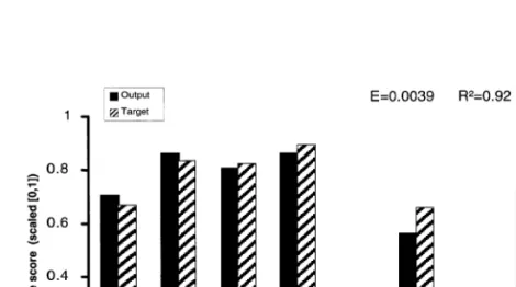
was reached for the average score of the seven hydromorphological variables — in Germany, the assessment used for the morphological structure of streams is called Gewa¨sserstruktur-Gu¨teklasse (Fig. 2).
3.3. Population dynamics of aquatic insects The results of CCA-ordination indicated a strong dependence of the population density ofA. fimbriata on the discharge pattern (Wagner and Schmidt, 1999). Abundance was highest at high discharge with low flow variability (D), was lower at winter and spring floods (E), and lowest during periods of low flow (F) or after seasonally unpre-dictable discharge events (B in Fig. 3). Based on monthly data, no significant dependence of D–P was detected. Abundance between patterns was significantly different. However, predictions could only be made with an error of hundreds of speci-mens per year.
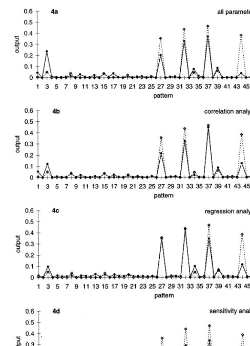
The precision of the ANN model with the original data was quite high (R2=0.63).
All months with any abundance were predicted correctly. The abundance magnitude differed between prediction and actual data (Fig. 4a). Pre-selection of five variables (abundance0,
abundance11, temperature1, temperature6,
I . M . Schleiter et al . / Ecological Modelling 120 (1999) 271 – 286 278 Table 4
Generalisation error of 5-3-1-BPN and 5×5-FM for predictions of chemical parameters from the abundance of five macroinvertebrates at each case identified with regression analysis
Target parame- Oxygen Conductivity BOD5 NH4N pH ter FM BPN FM BPN FM BPN FM BPN FM BPN Network type Error 0.01029 0.00229 0.01227 b 0.00465 0.00631 0.00290a 0.01851 0.00836 0.00278 Minimum 0.01232 0.01006 0.01645 0.00971 0.01726 0.01678 0.03063 0.02241 0.02117 Maximum 0.01089 0.00682 0.00611 0.00887 0.00834 0.00943 0.01247 0.00710 0.01770 0.01479 0.01915 Mean 0.01159 0.00493 0.01524 0.01374 0.01851 0.00742 0.00872 0.00745 0.01013 Median 0.00562 2.95E-06
3.49E-06 3.76E-07 8.48E-06 5.64E-06 6.00E-06 1.86E-05 4.33E-05 1.71E-05 1.07E-06 Standard
devia-tion
Species Chironomus thummi-Gr Limnius6olckmari Agabussp. Sigara lateralis Glossiphonia complanata Dolichopodidae indet. Elmis sp. Dolichopodidae indet Dolichopodidae indet Radix peregra
Sericostomatidae indet.
Goera pilosa Goera pilos Limnodrilussp. Limnophilasp.
Tanytarsini indet. Sigara fossarum Hydroporussp. Oreodytes sanmarkii Calopteryx splendens
Chironomus plumosus-Gr Daphnia pulex Chironomus plumosus-Gr Nemoura a6icularis
Anacaena limbata Ptot NH3N COD Target parame- NO2N NO3N ter BPN FM BPN BPN FM BPN FM BPN FM Networktype FM Error 0.00970 0.00731 0.00899 0.00369 0.01212 0.00552 0.00970 0.00292 Minimum 0.02624 0.01634 0.02873 0.01830 0.02657 0.01412 0.02017 0.01566 Maximum 0.05646 0.03338 0.02264 0.01037 0.01518 0.00793 Mean 0.02708 0.03054 0.01930 0.01016 0.01103 0.02312 0.00890 0.01564 3.70E-06 4.89E-05 1.57E-05 3.11E-05 4.94E-06
5.58E-08 1.54E-05
Standard devia- 1.24E-04 6.70E-06 2.21E-06 tion
Gammarus pulex Ilybius fuliginosus Ilybius fuliginosus Culexsp. Chironomidae indet.
Species
Goera pilosa Limnephilus rhombicus Chironomussp.
Bathyomphalus contortus Enallagma cyathigerum
Radix auricularia Erpobdella octoculata Limnophilasp. Rhyacophilasp.
Dolichopodidae indet
Helobdella stagnalis Pyrrhosoma nymphula Sigarasp. Limnephilus rhombicus Tanytarsini indet.
Bathyomphalus contortus Culexsp. Tubifexsp. Hydropsyche angustipennis Chaetopteryx6illosa
the accuracy of the model toR2=0.86 (Fig. 4b).
Cross correlation indicated almost no influence of precipitation on A. fimbriata abundance. Pre-se-lection by regression analysis found other vari-ables relevant (abundance0, abundance10, abundance11, temperature1, precipitation12) and increased the accuracy of the model to R2=0.86
(Fig. 4c). The best of three different sensitivity analyses selected the variables abundance0,
abundance11, temperature0, temperature6,
discharge6, and had an accuracy of R2=0.93
(Fig. 4d). An overview of these experiments indi-cates the best models were computed with a pre-selection of the best five variables by sensitivity analysis or regression. The models with variables pre-selected by correlation or without any pre-se-lection resulted in lower measure of accuracy (Table 6). ANN models generally explained much
more variability (20 – 30%) than linear regression models.
4. Discussion
The corresponding chemical data of the previ-ous day proved to be the most important network input, when modelling water quality of the river Lahn. Using other or supplementary input vari-ables, we achieved no significant improvement of the generalisation performance of the networks. This result is attributed to the strong autocorrela-tion of the values at the time t and t+1.
In our experience, the most important basis for successful neural modelling is a sound and repre-sentative data base. For example, from our data it was not possible to predict the temporal variation
Fig. 1. Comparison of measured and modelled temporal patterns of oxygen based on daily sum of precipitation and oxygen (24 60-min-values) of the previous day with 25-8-24-BPN (151 daily data sets for training and test).
I.M.Schleiter et al./Ecological Modelling120 (1999) 271 – 286
280
Table 5
Modelling morphological habitat characteristics with 5-3-1-senso-nets from the abundance of five macroinvertebrates at each case identified with regression analysis
Target Error R2
min Species
0.87
Discharge regime 0.0067 Gammarus pulex Gammarus roeseli Nemoura cinerea Dolichopodidae indet. Agabus guttatus (I) 0.83
Width/depth ratio 0.009 Rhyacophila fasci
-ata
Dugesia gono
-cephala Tanypodinae in
-det.
Elmis aenea(I)
Agabus guttatus
(I)
Diversity of substrate 0.0132 0.82 Tanypodinae indet Gammarus pulex Agabus didymus Tubifexsp. Pilariasp. 0.64 0.0137 Chironomus Fine sediments thummi-Gr Gammarus pulex Tanypodinae in -det. Pilariasp. Agabus didymus 0.0096 0.83 Gammarus pulex Diversity of habitat features Pilariasp. Gyraulus albus Gyrinussp. Hydropsychesp. 0.0048 0.90 Rhyacophila fasci -Extension of riparian zone ata Electrogenasp. Ephemerella ignita Limnodrilussp. Sigarasp. 0.0048 0.95 Sericostomatidae Structure of river bank indet. Pilariasp. Hydropsyche an -gustipennis Plectrocnemia conspersa Dytiscidae indet.
of water quality as a function of meteorological data. For this purpose, precise data gathering or a spatial-temporal allocation of the input (radia-tion, precipitation) and target variables (e.g. oxy-gen) are necessary on compatible time scales.
Generally, whether the temporal dependence of output data is derived on a specific time scale or integrated over an indefinite period of time is decisive. Accordingly, different network ap-proaches, either (non-linear) auto-regression or (partial) recurrent networks (e.g. Jordan-nets; Pham and Oh, 1992), are more suitable for suc-cessful modelling. The time dependent integration of previous states and events/processes is a major problem when modelling time series. We expect better modelling with specific time-dependent net-works with feedback onto specific neurons storing internal network states.
Due to their specific features, particularly the ability to handle non-linearities, ANNs combined with specific procedures for the selection of input variables provide an attractive tool for modelling species/species traits and habitat relations. A se-ries of chemical and hydromorphological proper-ties could be modelled with low error from the abundance of only a few specific macroinverte-brates identified with regression analysis. This di-mension-reducing, pre-processing caused an increase of the generalisation performance of the networks and a considerable reduction of the calculation effort. The results clearly indicate functional relationships between colonisation pat-terns of benthic macroinvertebrates and chemical and hydromorphological habitat characteristics within lotic ecosystems. Furthermore, a hierarchy of factors determining the community structure of invertebrates may be identified from theoretically numerous impact variables.
The species groups selected for each chemical and morphological model showed no or little congruence (see Tables 4 and 5). Even for related variables, different species groups were detected. Some species were selected by several models (e.g. Gammarus pulex: discharge regime, diversity of habitat features, Ptot, diversity of substrate, fine sediments), whereas others appeared in only one model. Because of restrictions in the basic data set due to the narrow geographical region and limited
abiotic gradients, the selected species groups in our examples may not be generalized. The results obtained here need further analysis with ecologi-cal information and validation based on addi-tional data. Thereby more approaches have to be tested as genetic algorithms (Goldberg, 1989) to detect relevant predictors for non-linear models based on general regression neural networks (Specht, 1991), equation synthesis (e.g. Road-knight et al., 1997), weight analysis (Balls et al. 1996,) and correlated activity pruning (Wiersma et al., 1995). Based on more comprehensive data, we would expect it to be possible to verify if key species or species assemblages for definite abiotic environmental states can be identified indepen-dently and reproduced for different sites. This may also be possible using the species traits hy-pothesis (Resh et al., 1994).
Discharge and water temperature are two main abiotic factors controlling the structure and dy-namics of stream invertebrate populations (Ward and Stanford, 1979, 1982), as well as the variabil-ity of habitats and the reproductive success of lotic species through metabolic processes (e.g. Feminella and Resh, 1990; Ce´re´ghino and La-vandier, 1998). However, many interdependencies
between the environment and the species remain less well known. The long-term population dy-namics of aquatic insects could be meaningfully described with ANNs in addition to classical statistics. Regression and correlation models have repeatedly been used to explain patterns in com-munities and they provided useful insights on environmental control of ecosystems, but their predictive power is low (ter Braak and Verdon-schot, 1995; Paruelo and Tomasel, 1997; Walley and Fontama, 1998). With classical statistical methods and ordination (CCA; ter Braak, 1988, 1990), the variability between year abundance of individual species was attributed mainly to the discharge pattern during larval development (Wagner and Schmidt, 1999). Due to the necessity to recognise patterns and not single discharge events, ANNs are an alternative method to model species abundance (Colasanti, 1991; Lek et al., 1996).
Larvae of A. fimbriata are grazers that avoid sandy substratum, they undergo a dormancy from November to the next February underneath larger stones (Aurich, 1992). Concerning the life history traits, pattern D (Fig. 3) provided low discharge
Fig. 2. Modelling average score of seven hydromorphological parameters with 5-3-1-senso-nets from the abundance of five macroinvertebrates at each case identified with regression analysis.
I.M.Schleiter et al./Ecological Modelling120 (1999) 271 – 286
282
Fig. 3. Discharge patterns of the Breitenbach discriminated with CCA: (A) 25-years mean of monthly maximum discharge; (B) years with non-seasonal events; (C) the seasonal pattern; (D) permanent, good discharge; (E) winter and spring floods; (F) long-term low flow [mean of within group monthly maximum (line)91 SD (raster)], and the density (ind/5m2) ofA.fimbriataat patterns D, E,
F and B (top left).
variability for almost an entire year at high mean flow. Strongly increased discharge in winter and spring disturb larval populations in dormancy, and low flow conditions over almost the entire year are disadvantageous for the development of eggs in summer, larvae in dormancy, and the pupae in early summer, due to increased deposi-tion of organic or inorganic material. Lowest success at the non-seasonal pattern is interpreted as the interaction of the magnitude and the dura-tion of floods. Most other aquatic insects, with the exception of the mayflyBaetis6ernus(Curtis), have their lowest abundance at these discharge pattern (Wagner and Schmidt, 1999).
In ANN models the best pre-selection method was a sensitivity analysis, whereas other methods were less accurate in the prediction ofA.fimbriata abundance. B. 6ernus was also best modelled by sensitivity pre-selection, but in B. rhodani pre-se-lection by correlation was optimal (Wagner et al., 1999). Variables selected for the best models of all three species were abundance of the parent gener-ation and temperature during the emergence or oviposition period of the parents. In addition, in
A. fimbriata temperature and discharge 6 months before emergence are among the most relevant predictors. During this period larvae are in winter dormancy, and higher temperature or discharge may have disturbed the larvae or their habitat. This demonstrates the potential of precise abun-dance predictions some months before emergence of the adults, and of the preselection methods, in particular sensitivity analysis, that detected sensi-tive conditions or periods in the life cycle of A. fimbriata.
5. Conclusion and perspectives
The results show that ANNs can successfully and meaningfully be applied in the analysis of effect-relations (e.g. species/species traits with habitat) including the identification and assess-ment of complex impact factors and for the pre-diction of system behavior (e.g. critical water states with an early-warning-system and long-term population dynamics depending on
environ-mental variables) having specific features com-pared with conventional methods (see Werner et al., 1999). Particularly, they have advantages if the relationships are unknown, very complex or non-linear. Combined with specific procedures for
the selection of the most important impact vari-ables, they can be used to reduce the input dimen-sion and therefore the complexity in a reasonable way. This causes an increase of the generalisation performance and a simplification of the model
Fig. 4. Abundance prediction ofA.fimbriata. (4a) Model, all input-variables, best generalisation (lowest error): 51-10-1-senso-net; (4b – d) Model, pre-selection by different methods, best generalisation: 5-3-1-senso-net. (Model, full line, diamond; observed data, dotted line, square).
I.M.Schleiter et al./Ecological Modelling120 (1999) 271 – 286
284
Table 6
Overview of some ANN models with different network input modes to predict the abundance ofA.fimbriata
Sensonets, generalisation performance Pre-processing
R2
Errormin Errormean
0.63 All variables 0.0022 0.0040 0.86 Correlation 0.0010 0.0019 0.86 0.0009 0.0017 Regression 0.0010 Sensitivity 0.93 0.0020 References
Aurich, M., 1992. The life-cycle ofApatania fimbriataPictet in the Breitenbach. Hydrobiologia 239, 65 – 78.
Balls, G.R., Palmer-Brown, D., Sanders, G.E., 1996. Investi-gating microclimatic influences on ozone injury in clover (Trifolium subterraneum) using artificial neural networks. N. Phyto. 132, 271 – 280.
Bayerisches Landesamt fu¨r Wasserwirtschaft (Hrsg.), 1998. Integrierte o¨kologische Gewa¨sserbewertung — Inhalte und Mo¨glichkeiten. Mu¨nch. Beitr. Abwasser Fisch. Flußbiol. 51, 683.
Borchardt, D., Dapper, T., Schleiter, I., Schmidt, K.-D., Werner, H., Wagner, R., 1997. Modellierung von Wirkungszusammenha¨ngen in Fließgewa¨ssern mit Hilfe Neuronaler Netzwerke. Abschlußbericht zum DFG-Forschungsvorhaben We 959/5-2, Universita¨t-Gh Kassel, pp. 141.
Ce´re´ghino, R., Lavandier, P., 1998. Influence of hypolimnetic hydropeaking on the distribution and population dynamics of Ephemeroptera in a mountain stream. Freshw. Biol. 40, 385 – 399.
Chon, T.-S., Park, Y.S., Moon, K.H., Cha, E.Y., 1996. Patt-ernizing communities by using an artificial neural network. Ecol. Model. 90, 69 – 78.
Colasanti, R.L., 1991. Discussions of the possible use of neural network algorithms in ecological modelling. Comput. Mi-crobiol. 3, 13 – 15.
Daniell, T.M., Wundke, A.D., 1993. Neural Networks — As-sisting in Water Quality Modelling. Watercomp, Mel-bourne, Australia, March 30 – April 1, Internal report, pp. 51 – 57.
Dapper, T., 1998. Dimensionsreduzierende Vorverarbeitungen fu¨r Neuronale Netze mit Anwendungen in der Gewa¨ssero¨kologie. Dissertation im Fachbereich Mathe-matik/Informatik der Universita¨t Gh Kassel, Berichte aus der Informatik D 34, Shaker Verlag, Aachen, pp. 243. Feminella, J.W., Resh, V.H., 1990. Hydrologic influences,
disturbance, and intraspecific competition in a stream cad-disfly population. Ecology 71, 2083 – 2094.
Goldberg, D.E., 1989. Genetic Algorithms in Search, Opti-mization and Machine Learning. korr. Nachdruck d. 1. Auflage, Addison-Wesley, Reading MA, pp. 412. Gue´gan, J.-F., Lek, S., Oberdorff, T., 1998. Energy availability
and habitat heterogeneity global riverine fish diversity. Nature 391, 382 – 384.
Kaluli, J.W., Madramootoo, C.A., Djebbar, Y., 1998. Mod-elling nitrate leaching using neural networks. Water Sci. Technol. 38 (7), 127 – 134.
Lachtermacher, G., Fuller, J.D., 1994. Backpropagation in hydrological time series forcasting, in stochastic and statis-tical methods. In: Hipel, K.W., McLeod, A.I., Panu, U.S., Singh, V.P. (Eds.), Hydrology and Environmental Engi-neering. Kluwer Academy, Norwell, MA, pp. 229 – 242. Lee, H.-L., DeAngelis, D., Koh, H.-L., 1998. Modelling
spa-tial distribution of the unionid mussels and the core-satel-lite hypothesis. Water Sci. Technol. 38 (7), 73 – 79.
and allows a better understanding of the under-lying relations.
Because the networks learn from examples, the quality of the neural models heavily depends on the quality of the data base, in particular whether it is representative for the given prob-lem, the given site or the given study period. Therefore, representative and compatible data are the main requirement for neural models.
We expect that with the aid of neural models and specific dimension-reducing, pre-processing methods, bioindication, ecological prediction and the analysis of cause-effect-relations can be im-proved substantially. Generally, modelling com-plex non-linear relationships can be handled considerably better with ANNs and supplemen-tary modelling techniques than with classical methods. The best results may be obtained with specific combinations of linear and non-linear techniques.
Acknowledgements
This study was supported by a grant through the German Research Foundation (Deutsche Forschungsgemeinschaft) to D. Borchardt (BO 1012). Numerous assistants and students have contributed for many years in the collection and determination of the insects and the preparation of the data, particularly E. Do¨ring, H. Quast-Fiebig, G. Stu¨ber, E. Turba, B. Landvogt-Pi-esche. M. Obach assisted in the revision and prepared Fig. 4. T. Horvath provided linguistic advice. All this help is gratefully acknowledged.
Lek, S., Belaud, A., Baran, P., Dimopoulos, I., Delacoste, M., 1996. Role of some environmental variables in trout abun-dance models using neural networks. Aquat. Living Re-sour. 9, 23 – 29.
Maier, H.R., 1995a. Use of artificial neural networks for modelling multivariate water quality time series. PhD The-sis. Department of Civil and Environmental Engineering, The University of Adelaide, pp. 464.
Maier, H.R., 1995b. A review of artificial neural networks. Research Report No. R131. Department of Civil and Environmental Engineering, The University of Adelaide, Adelaide, pp. 94.
Maier, H.R., Dandy, G.C., 1993. Use of Artificial neural networks for forecasting water quality. Reprints, Stochas-tic and StatisStochas-tical Methods in Hydrology and Environmen-tal Engineering. An International Conference in Honour of Professor T.E. Unny, University of Waterloo, Ont., Canada, June, 21 – 25, pp. 509 – 511.
Maier, H.R., Dandy, G.C., 1994. Forecasting salinity using neural networks and multivariate time series models. Reprints, Water Down Under 94, Adelaide, South Aus-tralia, November 21 – 25, pp. 297 – 302.
Maier, H.R., Dandy, G.C., 1996a. Neural network models for forecasting univariate time series. Neural Netw. World 5 (96), 747 – 771.
Maier, H.R., Dandy, G.C., 1996b. The use of artificial neural networks for the prediction of water quality parameters. Water Resour. Res. 32 (4), 1013 – 1022.
Maier, H.R., Dandy, G.C., Burch, M.D., 1998. Use of artifi-cial neural networks for modelling cyanobacteriaAnabena
spp. in the River Murray, South Australia. Ecol. Model. 105, 257 – 272.
Mang, J., Geffers, K., Borchardt, D., 1998. Fallbeispiel Lahn bei Limburg (Hessen) — ein staureguliertes Fließgewa¨sser 2. Ordnung. gwf-Wasser Abfall 139 (7), 408 – 417.
Paruelo, J.M., Tomasel, F., 1997. Prediction of functional characteristics of ecosystems — a comparison of artificial neural networks and regression models. Ecol. Model. 98, 73 – 186.
Pham, D.T., Oh, S.J., 1992. A recurrent backpropagation neural network for dynamic system identification. J. Syst. Eng. 2, 213 – 223.
Recknagel, F., 1997. ANNA — artificial neural network model for predicting species abundance and succession of blue – green algae. Hydrobiologia 349, 47 – 57.
Recknagel, F., French, M., Harkonen, P., Yabunaka, K.-I., 1997. Artificial neural network approach for modelling and prediction of algal blooms. Ecol. Model. 96, 11 – 28. Recknagel, F., Fukushima, T., Hanazato, T., Takamura, N.,
Wilson, H., 1998. Modelling and prediction of phyto- and zooplankton dynamics in Lake Kasumigaura by artificial neural networks. Lakes Reserv. Res. Manag. 3, 123 – 133. Resh, V.H., Hildrew, A.G., Statzner, B., Townsed, C.R., 1994.
Theoretical habitat templets, species traits, and species richness: a sysnthesis of long-term ecological research on the Upper Rhoˆne River in the context of concurrently developed ecological theory. Freshw. Biol. 31, 539 – 554.
Ritter, H., Martinez, T., Schulten, K., 1994. Neuronale Netze: eine Einfuehrung in die Neuroinformatik selbstorgan-isierender Netzwerke (2. Aufl.). Addison-Wesley, Bonn, pp. 325.
Roadknight, C.M., Balls, G.R., Mills, G.E., Palmer-Brown, D., 1997. Modelling complex environmental data. IEEE Trans. Neural Netw. 8, 852 – 862.
Rumelhart, D.E., Hinton, G.E., Williams, R.J., 1986. Learn-ing internal representations by error propagation. In: Rumelhart, D.E., McChelland, J.L. (Eds.), Parallel Dis-tributed Processing, vol. 1. MIT, Cambridge, MA, p. 318. Schizas, C.N., Pattiches, C.S, Michaelides, S.C., 1994. Fore-casting minimum temperature with short time-length data using artificial neural networks. Neural Netw. World 4 (2), 219 – 230.
Specht, D.F., 1991. A general regression network. IEEE Trans. Neural Netw. 6, 568 – 576.
SPSS Inc., 1997. SPSS for Windows, Base system user’s guide, Release 7.5.1., Chicago, USA, pp. 628.
Statzner, B., Gore, J.A., Resh, V.C., 1988. Hydraulic stream ecology: observed patterns and potential applications. J. N. Am. Benthol. Soc. 7, 307 – 360.
Statzner, B., Resh, V.H., Dole´dec, S. (Eds.), 1994. Ecology of the upper Rhoˆne River: a test of habitat templet theories. Special issue. Freshw. Biol. 31 (3), 556.
ter Braak, C.J.F., Verdonschot, P.F.M., 1995. Canonical cor-respondence analysis and related multivariate methods in aquatic ecology. Aquat. Sci. 57, 255 – 289.
ter Braak, C.J.F., 1988. CANOCO — a Fortran program for canonical community ordination by [partial] [detrended] [canonical] correspondence analysis, principal component analysis and redundancy analysis (version 2.1). Agricul-tural Mathematics Group, Wageningen, The Netherlands, pp. 95.
ter Braak, C.J.F., 1990. Update notes, CANOCO version 3.10. Agricultural Mathematics Group, Wageningen, The Netherlands, pp. 35.
Townsend, C.R., 1989. The patch dynamics concept of stream community ecology. J. North Am. Benthol. Soc. 8, 36 – 50. Townsend, C.R., Hildrew, A.G., 1994. Species traits in rela-tion to a habitat templet for river systems. Freshw. Biol. 31, 265 – 275.
Vannote, R.L., Minshall, G.W., Cummins, K.W., Sedell, J.R., Cushing, C.E., 1980. The river continuum concept. Can. J. Fish. Aquat. Sci. 37, 130 – 137.
Wagner, R., Dapper, T., Schmidt, H.-H., 1999. The influence of environmental variables on the abundance of aquatic insects — a comparison of ordination and artificial neural networks. Hydrobiologia (in press).
Wagner, R., Schmidt, H.-H. Relationship of aquatic insects emergence (Ephemeroptera,Plecoptera,Trichoptera) to en-vironmental variables: a 25 years analysis of the breiten-bach. Freshw. Biol. (in preparation).
Walley, W.J., Fontama, V.N., 1998. Neural network predic-tors of average score per taxon and number of families at unpolluted river sites in Great Britain. Water Res. 32, 613 – 622.
I.M.Schleiter et al./Ecological Modelling120 (1999) 271 – 286
286
Ward, J.V., Stanford, J.A., 1979. Ecological factors con-trolling stream zoobenthos with emphasis on thermal mod-ifications of regulated streams. In: Ward, J.V., Stanford, J.A. (Eds.), The ecology of regulated streams. Plenum, New York, pp. 35 – 55.
Ward, J.V., Stanford, J.A., 1982. Thermal responses in the evolutionary ecology of aquatic insects. Ann. Rev. Ento-mol. 27, 97 – 117.
Wen, C.-G., Lee, C.-S., 1998. A neural network approach to multiobjective optimization for water quality man-agement in a river basin. Water Resour. Res. 34, 427 – 436.
Werner, H., Dapper, T., Schmidt, K.-D., Borchardt, D., Schleiter, I.M., Wagner, R., Schmidt, H.-H., 1999. In: Neural network tools for the analysis of ecological data aquatic systems. (In preparation)
Wiersma, F.R., Poel, M., Oudshoff, A.M., 1995. The BB neural network rule extraction method. In: Kappen, B., Gielen, S. (Eds.), Proceedings of the 3rd Annual SNN Symposium on Neural Networks. Springer-Verlag, pp. 69 – 73.
Winkler, U., Voigtla¨nder, G., 1995. Anwendung neuronaler Netze fu¨r die Simulation von Prozeßabla¨ufen auf vorhan-denen Kla¨ranlagen. Korrespond. Abwasser 10, 1784 – 1792.
. .