Data Mining In Excel: Lecture Notes and Cases
Draft December 30, 2005
Galit Shmueli
Nitin R. Patel
Peter C. Bruce
(c) 2005 Galit Shmueli, Nitin R. Patel, Peter C. Bruce
Distributed by: Resampling Stats, Inc.
612 N. Jackson St. Arlington, VA 22201
USA [email protected] www.xlminer.com
Contents
1 Introduction 1
1.1 Who Is This Book For? . . . 1
1.2 What Is Data Mining? . . . 2
1.3 Where Is Data Mining Used? . . . 3
1.4 The Origins of Data Mining . . . 3
1.5 The Rapid Growth of Data Mining . . . 4
1.6 Why are there so many different methods? . . . 5
1.7 Terminology and Notation . . . 5
1.8 Road Maps to This Book . . . 7
2 Overview of the Data Mining Process 9 2.1 Introduction . . . 9
2.2 Core Ideas in Data Mining . . . 9
2.2.1 Classification . . . 9 2.2.2 Prediction . . . 9 2.2.3 Association Rules . . . 10 2.2.4 Predictive Analytics . . . 10 2.2.5 Data Reduction . . . 10 2.2.6 Data Exploration . . . 10 2.2.7 Data Visualization . . . 10
2.3 Supervised and Unsupervised Learning . . . 11
2.4 The Steps in Data Mining . . . 11
2.5 Preliminary Steps . . . 12
2.5.1 Organization of Datasets . . . 12
2.5.2 Sampling from a Database . . . 13
2.5.3 Oversampling Rare Events . . . 13
2.5.4 Pre-processing and Cleaning the Data . . . 13
2.5.5 Use and Creation of Partitions . . . 18
2.6 Building a Model - An Example with Linear Regression . . . 20
2.7 Using Excel For Data Mining . . . 27
2.8 Exercises . . . 30
3 Data Exploration and Dimension Reduction 33 3.1 Introduction . . . 33
3.2 Practical Considerations . . . 33
3.3 Data Summaries . . . 34
3.4 Data Visualization . . . 36
3.5 Correlation Analysis . . . 38
3.6 Reducing the Number of Categories in Categorical Variables . . . 39 i
ii CONTENTS
3.7 Principal Components Analysis . . . 39
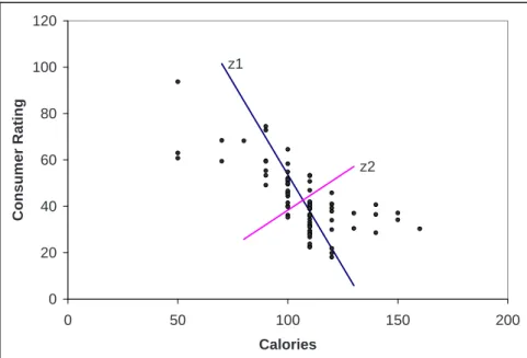
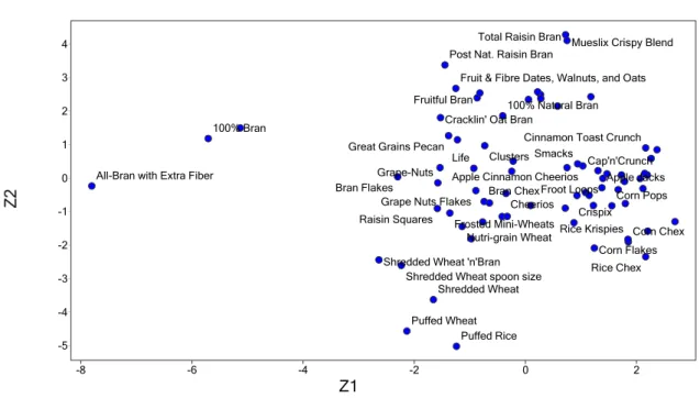
3.7.1 Example 2: Breakfast Cereals . . . 39
3.7.2 The Principal Components . . . 43
3.7.3 Normalizing the Data . . . 44
3.7.4 Using Principal Components for Classification and Prediction . . . 46
3.8 Exercises . . . 47
4 Evaluating Classification and Predictive Performance 49 4.1 Introduction . . . 49
4.2 Judging Classification Performance . . . 49
4.2.1 Accuracy Measures . . . 49
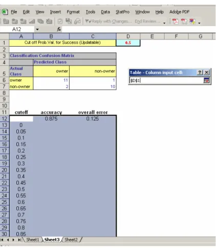
4.2.2 Cutoff For Classification . . . 52
4.2.3 Performance in Unequal Importance of Classes . . . 55
4.2.4 Asymmetric Misclassification Costs . . . 59
4.2.5 Oversampling and Asymmetric Costs . . . 62
4.2.6 Classification Using a Triage Strategy . . . 67
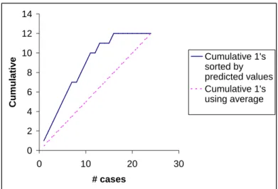
4.3 Evaluating Predictive Performance . . . 68
4.4 Exercises . . . 70
5 Multiple Linear Regression 73 5.1 Introduction . . . 73
5.2 Explanatory Vs. Predictive Modeling . . . 73
5.3 Estimating the Regression Equation and Prediction . . . 74
5.3.1 Example: Predicting the Price of Used Toyota Corolla Automobiles . . . 75
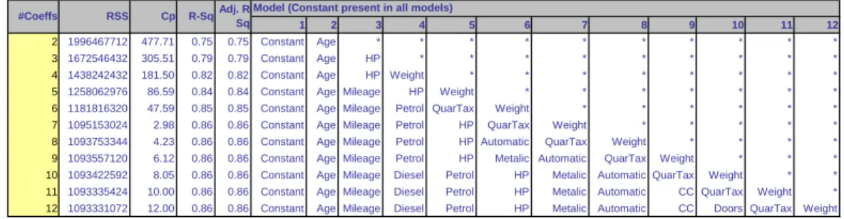
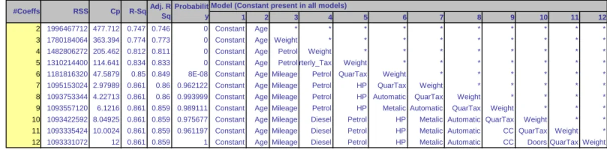
5.4 Variable Selection in Linear Regression . . . 78
5.4.1 Reducing the Number of Predictors . . . 78
5.4.2 How to Reduce the Number of Predictors . . . 79
5.5 Exercises . . . 83
6 Three Simple Classification Methods 87 6.1 Introduction . . . 87
6.1.1 Example 1: Predicting Fraudulent Financial Reporting . . . 87
6.1.2 Example 2: Predicting Delayed Flights . . . 88
6.2 The Naive Rule . . . 88
6.3 Naive Bayes . . . 89
6.3.1 Bayes Theorem . . . 89
6.3.2 A Practical Difficulty and a Solution: From Bayes to Naive Bayes . . . 90
6.3.3 Advantages and Shortcomings of the Naive Bayes Classifier . . . 94
6.4 k-Nearest Neighbor (k-NN) . . . . 97
6.4.1 Example 3: Riding Mowers . . . 98
6.4.2 Choosingk . . . 99
6.4.3 k-NN for a Quantitative Response . . . . 100
6.4.4 Advantages and Shortcomings of k-NN Algorithms . . . 100
6.5 Exercises . . . 102
7 Classification and Regression Trees 105 7.1 Introduction . . . 105
7.2 Classification Trees . . . 105
7.3 Recursive Partitioning . . . 105
7.4 Example 1: Riding Mowers . . . 106
7.4.1 Measures of Impurity . . . 108
CONTENTS iii
7.5.1 Example 2: Acceptance of Personal Loan . . . 113
7.6 Avoiding Overfitting . . . 114
7.6.1 Stopping Tree Growth: CHAID . . . 117
7.6.2 Pruning the Tree . . . 117
7.7 Classification Rules from Trees . . . 122
7.8 Regression Trees . . . 122
7.8.1 Prediction . . . 122
7.8.2 Measuring Impurity . . . 125
7.8.3 Evaluating Performance . . . 125
7.9 Advantages, Weaknesses, and Extensions . . . 125
7.10 Exercises . . . 127
8 Logistic Regression 131 8.1 Introduction . . . 131
8.2 The Logistic Regression Model . . . 132
8.2.1 Example: Acceptance of Personal Loan . . . 133
8.2.2 A Model with a Single Predictor . . . 135
8.2.3 Estimating the Logistic Model From Data: Computing Parameter Estimates 137 8.2.4 Interpreting Results in Terms of Odds . . . 139
8.3 Why Linear Regression is Inappropriate for a Categorical Response . . . 140
8.4 Evaluating Classification Performance . . . 140
8.4.1 Variable Selection . . . 143
8.5 Evaluating Goodness-of-Fit . . . 143
8.6 Example of Complete Analysis: Predicting Delayed Flights . . . 145
8.7 Logistic Regression for More than 2 Classes . . . 153
8.7.1 Ordinal Classes . . . 153
8.7.2 Nominal Classes . . . 154
8.8 Exercises . . . 155
9 Neural Nets 159 9.1 Introduction . . . 159
9.2 Concept and Structure of a Neural Network . . . 159
9.3 Fitting a Network to Data . . . 160
9.3.1 Example 1: Tiny Dataset . . . 160
9.3.2 Computing Output of Nodes . . . 161
9.3.3 Preprocessing the Data . . . 163
9.3.4 Training the Model . . . 164
9.3.5 Example 2: Classifying Accident Severity . . . 167
9.3.6 Using the Output for Prediction and Classification . . . 169
9.4 Required User Input . . . 173
9.5 Exploring the Relationship Between Predictors and Response . . . 174
9.6 Advantages and Weaknesses of Neural Networks . . . 174
9.7 Exercises . . . 175
10 Discriminant Analysis 177 10.1 Introduction . . . 177
10.2 Example 1: Riding Mowers . . . 177
10.3 Example 2: Personal Loan Acceptance . . . 177
10.4 Distance of an Observation from a Class . . . 178
10.5 Fisher’s Linear Classification Functions . . . 180
iv CONTENTS
10.7 Prior Probabilities . . . 185
10.8 Unequal Misclassification Costs . . . 185
10.9 Classifying More Than Two Classes . . . 186
10.9.1 Example 3: Medical Dispatch to Accident Scenes . . . 186
10.10Advantages and Weaknesses . . . 188
10.11Exercises . . . 190
11 Association Rules 193 11.1 Introduction . . . 193
11.2 Discovering Association Rules in Transaction Databases . . . 193
11.3 Example 1: Synthetic Data on Purchases of Phone Faceplates . . . 195
11.4 Generating Candidate Rules . . . 195
11.4.1 The Apriori Algorithm . . . 196
11.5 Selecting Strong Rules . . . 196
11.5.1 Support and Confidence . . . 196
11.5.2 Lift Ratio . . . 197
11.5.3 Data Format . . . 197
11.5.4 The Process of Rule Selection . . . 198
11.5.5 Interpreting the Results . . . 200
11.5.6 Statistical Significance of Rules . . . 200
11.6 Example 2: Rules for Similar Book Purchases . . . 201
11.7 Summary . . . 202
11.8 Exercises . . . 204
12 Cluster Analysis 207 12.1 Introduction . . . 207
12.2 Example: Public Utilities . . . 208
12.3 Measuring Distance Between Two Records . . . 208
12.3.1 Euclidean Distance . . . 210
12.3.2 Normalizing Numerical Measurements . . . 210
12.3.3 Other Distance Measures for Numerical Data . . . 211
12.3.4 Distance Measures for Categorical Data . . . 213
12.3.5 Distance Measures for Mixed Data . . . 214
12.4 Measuring Distance Between Two Clusters . . . 214
12.5 Hierarchical (Agglomerative) Clustering . . . 216
12.5.1 Minimum Distance (Single Linkage) . . . 216
12.5.2 Maximum Distance (Complete Linkage) . . . 217
12.5.3 Group Average (Average Linkage) . . . 217
12.5.4 Dendrograms: Displaying Clustering Process and Results . . . 217
12.5.5 Validating Clusters . . . 217
12.5.6 Limitations of Hierarchical Clustering . . . 220
12.6 Non-Hierarchical Clustering: Thek-Means Algorithm . . . . 221
12.6.1 Initial Partition IntokClusters . . . 222
12.7 Exercises . . . 225
13 Cases 227 13.1 Charles Book Club . . . 227
13.2 German Credit . . . 235
13.3 Tayko Software Cataloger . . . 239
13.4 Segmenting Consumers of Bath Soap . . . 244
CONTENTS v
13.6 Catalog Cross-Selling . . . 251
Chapter 1
Introduction
1.1
Who Is This Book For?
This book arose out of a data mining course at MIT’s Sloan School of Management. Preparation for the course revealed that there are a number of excellent books on the business context of data mining, but their coverage of the statistical and machine-learning algorithms that underlie data mining is not sufficiently detailed to provide a practical guide if the instructor’s goal is to equip students with the skills and tools to implement those algorithms. On the other hand, there are also a number of more technical books about data mining algorithms, but these are aimed at the statistical researcher, or more advanced graduate student, and do not provide the case-oriented business focus that is successful in teaching business students.
Hence, this book is intended for the business student (and practitioner) of data mining tech-niques, and its goal is threefold:
1. To provide both a theoretical and practical understanding of the key methods of classification, prediction, reduction and exploration that are at the heart of data mining;
2. To provide a business decision-making context for these methods;
3. Using real business cases, to illustrate the application and interpretation of these methods. An important feature of this book is the use of Excel, an environment familiar to business an-alysts. All required data mining algorithms (plus illustrative datasets) are provided in an Excel add-in, XLMiner. XLMiner offers a variety of data mining tools: neural nets, classification and regression trees, k-nearest neighbor classification, naive Bayes, logistic regression, multiple linear regression, and discriminant analysis, all for predictive modeling. It provides for automatic parti-tioning of data into training, validation and test samples, and for the deployment of the model to new data. It also offers association rules, principal components analysis, k-means clustering and hierarchical clustering, as well as visualization tools, and data handling utilities. With its short learning curve, affordable price, and reliance on the familiar Excel platform, it is an ideal companion to a book on data mining for the business student.
The presentation of the cases in the book is structured so that the reader can follow along and implement the algorithms on his or her own with a very low learning hurdle.
Just as a natural science course without a lab component would seem incomplete, a data mining course without practical work with actual data is missing a key ingredient. The MIT data mining course that gave rise to this book followed an introductory quantitative course that relied on Excel – this made its practical work universally accessible. Using Excel for data mining seemed a natural progression.
2 1. Introduction While the genesis for this book lay in the need for a case-oriented guide to teaching data mining, analysts and consultants who are considering the application of data mining techniques in contexts where they are not currently in use will also find this a useful, practical guide.
Using XLMiner Software
This book is based on using the XLMiner software. The illustrations, exercises, and cases are written with relation to this software. XLMiner is a comprehensive data mining add-in for Excel, which is easy to learn for users of Excel. It is a tool to help you get quickly started on data mining, offering a variety of methods to analyze data. It has extensive coverage of statistical and data mining techniques for classification, prediction, affinity analysis, and data exploration and reduction.
Installation: Click on setup.exe and installation dialog boxes will guide you through the instal-lation procedure. After instalinstal-lation is complete, the XLMiner program group appears under Start→ Programs→XLMiner. You can either invoke XLMiner directly or select the option to register XLMiner as an Excel Add-in.
Use: Once opened, XLMiner appears as another menu in the top toolbar in
Ex-cel, as shown in the figure below. By choosing the appropriate menu item, you can
run any of XLMiner’s procedures on the dataset that is open in the Excel worksheet.
Page 1 of 1
12/22/2005
http://www.resample.com/xlminer/help/GettingStarted/XLMiner1.gif
1.2
What Is Data Mining?
The field of data mining is still relatively new, and in a state of evolution. The first International Conference on Knowledge Discovery and Data Mining (“KDD”) was held in 1995, and there are a variety of definitions of data mining.
A concise definition that captures the essence of data mining is:
1.3. WHERE IS DATA MINING USED? 3
A slightly longer version is:
“Data mining is the process of exploration and analysis, by automatic or semi-automatic means, of large quantities of data in order to discover meaningful patterns and rules” (Berry and Linoff: 1997 and 2000).
Berry and Linoff later had cause to regret the 1997 reference to “automatic and semi-automatic means,” feeling it shortchanged the role of data exploration and analysis.
Another definition comes from the Gartner Group, the information technology research firm (from their web site, Jan. 2004):
“Data mining is the process of discovering meaningful new correlations, patterns and trends by sifting through large amounts of data stored in repositories, using pattern recognition technologies as well as statistical and mathematical techniques.”
A summary of the variety of methods encompassed in the term “data mining” is found at the beginning of Chapter 2 (Core Ideas).
1.3
Where Is Data Mining Used?
Data mining is used in a variety of fields and applications. The military use data mining to learn what roles various factors play in the accuracy of bombs. Intelligence agencies might use it to determine which of a huge quantity of intercepted communications are of interest. Security specialists might use these methods to determine whether a packet of network data constitutes a threat. Medical researchers might use them to predict the likelihood of a cancer relapse.
Although data mining methods and tools have general applicability, most examples in this book are chosen from the business world. Some common business questions one might address through data mining methods include:
1. From a large list of prospective customers, which are most likely to respond? We can use classification techniques (logistic regression, classification trees or other methods) to identify those individuals whose demographic and other data most closely matches that of our best existing customers. Similarly, we can use prediction techniques to forecast how much individual prospects will spend.
2. Which customers are most likely to commit, for example, fraud (or might already have commit-ted it)? We can use classification methods to identify (say) medical reimbursement applications that have a higher probability of involving fraud, and give them greater attention.
3. Which loan applicants are likely to default? We can use classification techniques to identify them (or logistic regression to assign a “probability of default” value).
4. Which customers are more likely to abandon a subscription service (telephone, magazine, etc.)? Again, we can use classification techniques to identify them (or logistic regression to assign a “probability of leaving” value). In this way, discounts or other enticements can be proffered selectively.
1.4
The Origins of Data Mining
Data mining stands at the confluence of the fields of statistics and machine learning (also known as artificial intelligence). A variety of techniques for exploring data and building models have been around for a long time in the world of statistics - linear regression , logistic regression, discriminant
4 1. Introduction analysis and principal components analysis, for example. But the core tenets of classical statistics-computing is difficult and data are scarce - do not apply in data mining applications where both data and computing power are plentiful.
This gives rise to Daryl Pregibon’s description of data mining as “statistics at scale and speed” (Pregibon, 1999). A useful extension of this is “statistics at scale, speed, and simplicity.” Simplicity in this case refers not to simplicity of algorithms, but rather to simplicity in the logic of inference. Due to the scarcity of data in the classical statistical setting, the same sample is used to make an estimate, and also to determine how reliable that estimate might be. As a result, the logic of the confidence intervals and hypothesis tests used for inference may seem elusive for many, and their limitations are not well appreciated. By contrast, the data mining paradigm of fitting a model with one sample and assessing its performance with another sample is easily understood.
Computer science has brought us “machine learning” techniques, such as trees and neural net-works , that rely on computational intensity and are less structured than classical statistical models. In addition, the growing field of database management is also part of the picture.
The emphasis that classical statistics places on inference (determining whether a pattern or interesting result might have happened by chance) is missing in data mining. In comparison to statistics, data mining deals with large datasets in open-ended fashion, making it impossible to put the strict limits around the question being addressed that inference would require.
As a result, the general approach to data mining is vulnerable to the danger of “overfitting,” where a model is fit so closely to the available sample of data that it describes not merely structural characteristics of the data, but random peculiarities as well. In engineering terms, the model is fitting the noise, not just the signal.
1.5
The Rapid Growth of Data Mining
Perhaps the most important factor propelling the growth of data mining is the growth of data. The mass retailer Walmart in 2003 captured 20 million transactions per day in a 10-terabyte database (a terabyte is 1,000,000 megabytes). In 1950, the largest companies had only enough data to occupy, in electronic form, several dozen megabytes. Lyman and Varian (2003) estimate that 5 exabytes of information were produced in 2002, double what was produced in 1999 (an exabyte is one million terabytes). 40% of this was produced in the U.S.
The growth of data is driven not simply by an expanding economy and knowledge base, but by the decreasing cost and increasing availability of automatic data capture mechanisms. Not only are more events being recorded, but more information per event is captured. Scannable bar codes, point of sale (POS) devices, mouse click trails, and global positioning satellite (GPS) data are examples.
The growth of the internet has created a vast new arena for information generation. Many of the same actions that people undertake in retail shopping, exploring a library or catalog shopping have close analogs on the internet, and all can now be measured in the most minute detail.
In marketing, a shift in focus from products and services to a focus on the customer and his or her needs has created a demand for detailed data on customers.
The operational databases used to record individual transactions in support of routine business activity can handle simple queries, but are not adequate for more complex and aggregate analysis. Data from these operational databases are therefore extracted, transformed and exported to adata warehouse - a large integrated data storage facility that ties together the decision support systems of an enterprise. Smaller data marts devoted to a single subject may also be part of the system. They may include data from external sources (e.g., credit rating data).
Many of the exploratory and analytical techniques used in data mining would not be possible without today’s computational power. The constantly declining cost of data storage and retrieval has made it possible to build the facilities required to store and make available vast amounts of data. In short, the rapid and continuing improvement in computing capacity is an essential enabler of the
1.6. WHY ARE THERE SO MANY DIFFERENT METHODS? 5
growth of data mining.
1.6
Why are there so many different methods?
As can be seen in this book or any other resource on data mining, there are many different methods for prediction and classification. You might ask yourself why they coexist, and whether some are better than others. The answer is that each method has its advantages and disadvantages. The usefulness of a method can depend on factors such as the size of the dataset, the types of patterns that exist in the data, whether the data meet some underlying assumptions of the method, how noisy the data are, the particular goal of the analysis, etc. A small illustration is shown in Figure 1.1, where the goal is to find a combination of household income level and household lot size that separate buyers (solid circles) from non-buyers (hollow circles) of riding mowers. The first method (left panel) looks only for horizontal and vertical lines to separate buyers from non-buyers, whereas the second method (right panel) looks for a single diagonal line.
13 15 17 19 21 23 25 20 40 60 80 100 120 Income ($000) L o t S ize ( 0 0 0 's s q ft ) owner non-owner 13 15 17 19 21 23 25 20 40 60 80 100 120 Income ($000) L o t S ize ( 0 0 0 's s q ft ) owner non-owner
Figure 1.1: Two different methods for separating buyers from non-buyers
Different methods can lead to different results, and their performance can vary. It is therefore customary in data mining to apply several different methods and select the one that is most useful for the goal at hand.
1.7
Terminology and Notation
Because of the hybrid parentry of data mining, its practitioners often use multiple terms to refer to the same thing. For example, in the machine learning (artificial intelligence) field, the variable being predicted is the output variable or the target variable. To a statistician, it is the dependent variable or the response. Here is a summary of terms used:
Algorithm refers to a specific procedure used to implement a particular data mining technique-classification tree, discriminant analysis, etc.
Attribute - seePredictor.
Case - seeObservation.
Confidence has a specific meaning in association rules of the type “If A and B are purchased, C is also purchased.” Confidence is the conditional probability that C will be purchased, IF A and B are purchased.
Confidence also has a broader meaning in statistics (“confidence interval”), concerning the degree of error in an estimate that results from selecting one sample as opposed to another.
6 1. Introduction
Dependent variable - seeResponse.
Estimation - seePrediction.
Feature - seePredictor.
Holdout sample is a sample of data not used in fitting a model, used to assess the performance of that model; this book uses the termsvalidation setor, if one is used in the problem,test set instead of holdout sample.
Input variable - seePredictor.
Model refers to an algorithm as applied to a dataset, complete with its settings (many of the algorithms have parameters which the user can adjust).
Observation is the unit of analysis on which the measurements are taken (a customer, a trans-action, etc.); also calledcase, record, patternor row. (each row typically represents a record, each column a variable)
Outcome variable - seeResponse.
Output variable - seeResponse.
P(A|B) is the conditional probability of eventA occurring given that eventB has occurred. Read as “the probability thatAwill occur, given thatB has occurred.”
Pattern is a set of measurements on an observation (e.g., the height, weight, and age of a person)
Prediction means the prediction of the value of a continuous output variable; also calledestimation.
Predictor usually denoted by X, is also called a feature,input variable, independent variable, or, from a database perspective, afield.
Record - see Observation.
Response , usually denoted byY, is the variable being predicted in supervised learning; also called dependent variable,output variable,target variableor outcome variable.
Score refers to a predicted value or class. “Scoring new data” means to use a model developed with training data to predict output values in new data.
Success class is the class of interest in a binary outcome (e.g., “purchasers” in the outcome “purchase/no-purchase”)
Supervised learning refers to the process of providing an algorithm (logistic regression, regression tree, etc.) with records in which an output variable of interest is known and the algorithm “learns” how to predict this value with new records where the output is unknown.
Test data (or test set) refers to that portion of the data used only at the end of the model building and selection process to assess how well the final model might perform on additional data.
Training data (or training set) refers to that portion of data used to fit a model.
Unsupervised learning refers to analysis in which one attempts to learn something about the data other than predicting an output value of interest (whether it falls into clusters, for example).
1.8. ROAD MAPS TO THIS BOOK 7
Data Preparation & Exploration (2-3) •Sampling •Cleaning •Summaries •Visualization •Partitioning •Dimension reduction Prediction · MLR (5) · K-nearest neighbor (6) · Regression trees (7) · Neural Nets (9) Classification · K-nearest neighbor (6) · Naive Bayes (6) · Logistic regression (8) · Classification trees (7) · Neural nets (9) · Discriminant analysis (10) Segmentation/ clustering (12) Affinity Analysis / Association Rules (11) Model evaluation & selection (4) Scoring new data Deriving insight
Figure 1.2: Data Mining From A Process Perspective
Validation data (or validation set) refers to that portion of the data used to assess how well the model fits, to adjust some models, and to select the best model from among those that have been tried.
Variable is any measurement on the records, including both the input (X) variables and the output (Y) variable.
1.8
Road Maps to This Book
The book covers many of the widely-used predictive and classification methods, as well as other data mining tools. Figure 1.2 outlines data mining from a process perspective, and where the topics in this book fit in. Chapter numbers are indicated beside the topic.
Table 1.1 provides a different perspective - what type of data we have, and what that says about the data mining procedures available.
Order of Topics
The chapters are generally divided into three parts: Chapters 1-3 cover general topics, Chapters 4-10 cover prediction and classification methods, and Chapters 11-12 discuss association rules and cluster analysis. Within the prediction and classification group of chapters, the topics are generally organized according to the level of sophistication of the algorithms, their popularity, and ease of understanding. Although the topics in the book can be covered in the order of the chapters, each chapter (aside from Chapters 1-4) stands alone so that it can be dropped or covered at a different time without loss in comprehension.
8 1. Introduction
Table 1.1: Organization Of Data Mining Methods In This Book, According To The Nature Of The Data
Continuous Response Categorical Response No Response
Continuous Predictors Linear Reg (5) Logistic Reg (8) Principal Components (3) Neural Nets (9) Neural Nets (9) Cluster Analysis (12) KNN (6) Discriminant Analysis (10)
KNN (6)
Categorical Predictors Linear Reg (5) Neural Nets (9) Association Rules (11) Neural Nets (9) Classification Trees (7)
Reg Trees (7) Logistic Reg (8) Naive Bayes (6)
Note: Chapter 3 (Data Exploration and Dimension Reduction) also covers principal components analysis as a method for dimension reduction. Instructors may wish to defer covering PCA to a later point.
Chapter 2
Overview of the Data Mining
Process
2.1
Introduction
In the previous chapter we saw some very general definitions of data mining. In this chapter we introduce the variety of methods sometimes referred to as “data mining.” The core of this book focuses on what has come to be called “predictive analytics” - the tasks of classification and prediction that are becoming key elements of a “Business Intelligence” function in most large firms. These terms are described and illustrated below.
Not covered in this book to any great extent are two simpler database methods that are some-times considered to be data mining techniques: (1) OLAP (online analytical processing) and (2) SQL (structured query language). OLAP and SQL searches on databases are descriptive in nature (“find all credit card customers in a certain zip code with annual charges>$20,000, who own their own home and who pay the entire amount of their monthly bill at least 95% of the time”) and do not involve statistical modeling.
2.2
Core Ideas in Data Mining
2.2.1
Classification
Classification is perhaps the most basic form of data analysis. The recipient of an offer can respond or not respond. An applicant for a loan can repay on time, repay late or declare bankruptcy. A credit card transaction can be normal or fraudulent. A packet of data traveling on a network can be benign or threatening. A bus in a fleet can be available for service or unavailable. The victim of an illness can be recovered, still ill, or deceased.
A common task in data mining is to examine data where the classification is unknown or will occur in the future, with the goal of predicting what that classification is or will be. Similar data where the classification is known are used to develop rules, which are then applied to the data with the unknown classification.
2.2.2
Prediction
Prediction is similar to classification, except we are trying to predict the value of a numerical variable (e.g., amount of purchase), rather than a class (e.g. purchaser or nonpurchaser).
10 2. Overview of the Data Mining Process Of course, in classification we are trying to predict a class, but the term “prediction” in this book refers to the prediction of the value of a continuous variable. (Sometimes in the data mining literature, the term “estimation” is used to refer to the prediction of the value of a continuous variable, and “prediction” may be used for both continuous and categorical data.)
2.2.3
Association Rules
Large databases of customer transactions lend themselves naturally to the analysis of associations among items purchased, or “what goes with what.” Association rules, oraffinity analysis can then be used in a variety of ways. For example, grocery stores can use such information after a customer’s purchases have all been scanned to print discount coupons, where the items being discounted are determined by mapping the customer’s purchases onto the association rules. Online merchants such as Amazon.com and Netflix.com use these methods as the heart of a “recommender” system that suggests new purchases to customers.
2.2.4
Predictive Analytics
Classification, prediction, and to some extent affinity analysis, constitute the analytical methods employed in “predictive analytics.”
2.2.5
Data Reduction
Sensible data analysis often requires distillation of complex data into simpler data. Rather than dealing with thousands of product types, an analyst might wish to group them into a smaller number of groups. This process of consolidating a large number of variables (or cases) into a smaller set is termed data reduction.
2.2.6
Data Exploration
Unless our data project is very narrowly focused on answering a specific question determined in advance (in which case it has drifted more into the realm of statistical analysis than of data mining), an essential part of the job is to review and examine the data to see what messages they hold, much as a detective might survey a crime scene. Here, full understanding of the data may require a reduction in its scale or dimension to allow us to see the forest without getting lost in the trees. Similar variables (i.e. variables that supply similar information) might be aggregated into a single variable incorporating all the similar variables. Analogously, records might be aggregated into groups of similar records.
2.2.7
Data Visualization
Another technique for exploring data to see what information they hold is through graphical analysis. This includes looking at each variable separately as well as looking at relationships between variables. For numeric variables we use histograms and boxplots to learn about the distribution of their values, to detect outliers (extreme observations), and to find other information that is relevant to the analysis task. Similarly, for categorical variables we use bar charts and pie charts. We can also look at scatter plots of pairs of numeric variables to learn about possible relationships, the type of relationship, and again, to detect outliers.
2.3. SUPERVISED AND UNSUPERVISED LEARNING 11
2.3
Supervised and Unsupervised Learning
A fundamental distinction among data mining techniques is between supervised methods and unsu-pervised methods.
“Supervised learning” algorithms are those used in classification and prediction. We must have data available in which the value of the outcome of interest (e.g. purchase or no purchase) is known. These “training data” are the data from which the classification or prediction algorithm “learns,” or is “trained,” about the relationship between predictor variables and the outcome variable. Once the algorithm has learned from the training data, it is then applied to another sample of data (the “validation data”) where the outcome is known, to see how well it does in comparison to other models. If many different models are being tried out, it is prudent to save a third sample of known outcomes (the “test data”) to use with the final, selected model to predict how well it will do. The model can then be used to classify or predict the outcome of interest in new cases where the outcome is unknown. Simple linear regression analysis is an example of supervised learning (though rarely called that in the introductory statistics course where you likely first encountered it). TheY variable is the (known) outcome variable and the X variable is some predictor variable. A regression line is drawn to minimize the sum of squared deviations between the actual Y values and the values predicted by this line. The regression line can now be used to predictY values for new values ofX for which we do not know theY value.
Unsupervised learning algorithms are those used where there is no outcome variable to predict or classify. Hence, there is no “learning” from cases where such an outcome variable is known. Association rules, data reduction methods and clustering techniques are all unsupervised learning methods.
2.4
The Steps in Data Mining
This book focuses on understanding and using data mining algorithms (steps 4-7 below). However, some of the most serious errors in data analysis result from a poor understanding of the problem -an underst-anding that must be developed before we get into the details of algorithms to be used. Here is a list of steps to be taken in a typical data mining effort:
1. Develop an understanding of the purpose of the data mining project (if it is a one-shot effort to answer a question or questions) or application (if it is an ongoing procedure).
2. Obtain the dataset to be used in the analysis. This often involves random sampling from a large database to capture records to be used in an analysis. It may also involve pulling together data from different databases. The databases could be internal (e.g. past purchases made by customers) or external (credit ratings). While data mining deals with very large databases, usually the analysis to be done requires only thousands or tens of thousands of records.
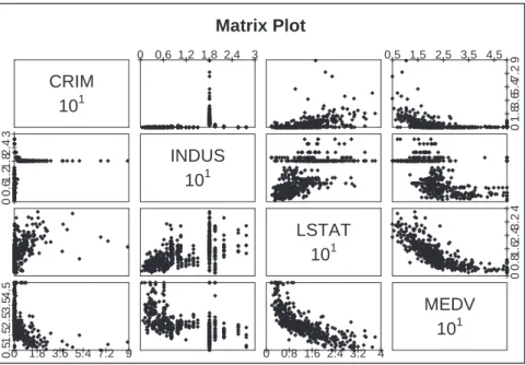
3. Explore, clean, and preprocess the data. This involves verifying that the data are in reasonable condition. How should missing data be handled? Are the values in a reasonable range, given what you would expect for each variable? Are there obvious “outliers?” The data are reviewed graphically - for example, a matrix of scatterplots showing the relationship of each variable with each other variable. We also need to ensure consistency in the definitions of fields, units of measurement, time periods, etc.
4. Reduce the data, if necessary, and (where supervised training is involved) separate them into training, validation and test datasets. This can involve operations such as eliminating unneeded variables, transforming variables (for example, turning “money spent” into “spent>$100” vs. “spent≤$100”), and creating new variables (for example, a variable that records whether at
12 2. Overview of the Data Mining least one of several products was purchased). Make sure you know what each variable means, and whether it is sensible to include it in the model.
5. Determine the data mining task (classification, prediction, clustering, etc.). This involves translating the general question or problem of step 1 into a more specific statistical question.
6. Choose the data mining techniques to be used (regression, neural nets, hierarchical clustering, etc.).
7. Use algorithms to perform the task. This is typically an iterative process - trying multiple variants, and often using multiple variants of the same algorithm (choosing different variables or settings within the algorithm). Where appropriate, feedback from the algorithm’s performance on validation data is used to refine the settings.
8. Interpret the results of the algorithms. This involves making a choice as to the best algorithm to deploy, and where possible, testing our final choice on the test data to get an idea how well it will perform. (Recall that each algorithm may also be tested on the validation data for tuning purposes; in this way the validation data becomes a part of the fitting process and is likely to underestimate the error in the deployment of the model that is finally chosen.)
9. Deploy the model. This involves integrating the model into operational systems and running it on real records to produce decisions or actions. For example, the model might be applied to a purchased list of possible customers, and the action might be “include in the mailing if the predicted amount of purchase is>$10.”
The above steps encompass the steps in SEMMA, a methodology developed by SAS: Sample: from datasets, partition into training, validation and test datasets
Explore: dataset statistically and graphically Modify: transform variables, impute missing values
Model: fit predictive models, e.g. regression, tree, collaborative filtering Assess: compare models using validation dataset
SPSS-Clementine also has a similar methodology, termed CRISP-DM (CRoss-Industry Standard Process for Data Mining).
2.5
Preliminary Steps
2.5.1
Organization of Datasets
Datasets are nearly always constructed and displayed so that variables are in columns, and records are in rows. In the example shown in Section 2.6 (the Boston Housing data), the values of 14 variables are recorded for a number of census tracts. The spreadsheet is organized such that each row represents a census tract - the first tract had a per capital crime rate (CRIM) of 0.00632, had 18% of its residential lots zoned for over 25,000 square feet (ZN), etc. In supervised learning situations, one of these variables will be the outcome variable, typically listed at the end or the beginning (in this case it is median value, MEDV, at the end).
2.5 Preliminary Steps 13
2.5.2
Sampling from a Database
Quite often, we want to perform our data mining analysis on less than the total number of records that are available. Data mining algorithms will have varying limitations on what they can handle in terms of the numbers of records and variables, limitations that may be specific to computing power and capacity as well as software limitations. Even within those limits, many algorithms will execute faster with smaller datasets.
From a statistical perspective, accurate models can often be built with as few as several hundred records (see below). Hence, we will often want to sample a subset of records for model building.
2.5.3
Oversampling Rare Events
If the event we are interested in is rare, however, (e.g. customers purchasing a product in response to a mailing), sampling a subset of records may yield so few events (e.g. purchases) that we have little information on them. We would end up with lots of data on non-purchasers, but little on which to base a model that distinguishes purchasers from non-purchasers. In such cases, we would want our sampling procedure to over-weight the purchasers relative to the non-purchasers so that our sample would end up with a healthy complement of purchasers. This issue arises mainly in classification problems because those are the types of problems in which an overwhelming number of 0’s is likely to be encountered in the response variable. While the same principle could be extended to prediction, any prediction problem in which most responses are 0 is likely to raise the question of what distinguishes responses from non-responses, i.e., a classification question. (For convenience below we speak of responders and non-responders, as to a promotional offer, but we are really referring to any binary - 0/1 - outcome situation.)
Assuring an adequate number of responder or “success” cases to train the model is just part of the picture. A more important factor is the costs of misclassification. Whenever the response rate is extremely low, we are likely to attach more importance to identifying a responder than identifying a non-responder. In direct response advertising (whether by traditional mail or via the internet), we may encounter only one or two responders for every hundred records - the value of finding such a customer far outweighs the costs of reaching him or her. In trying to identify fraudulent transactions, or customers unlikely to repay debt, the costs of failing to find the fraud or the non-paying customer are likely exceed the cost of more detailed review of a legitimate transaction or customer.
If the costs of failing to locate responders were comparable to the costs of misidentifying re-sponders as non-rere-sponders, our models would usually be at their best if they identified everyone (or almost everyone, if it is easy to pick off a few responders without catching many non-responders) as a non-responder. In such a case, the misclassification rate is very low - equal to the rate of responders - but the model is of no value.
More generally, we want to train our model with the asymmetric costs in mind, so that the algo-rithm will catch the more valuable responders, probably at the cost of “catching” and misclassifying more non-responders as responders than would be the case if we assume equal costs. This subject is discussed in detail in the next chapter.
2.5.4
Pre-processing and Cleaning the Data
Types of VariablesThere are several ways of classifying variables. Variables can be numeric or text (character). They can be continuous (able to assume any real numeric value, usually in a given range), integer (as-suming only integer values), or categorical (as(as-suming one of a limited number of values). Cate-gorical variables can be either numeric (1,2,3) or text (payments current, payments not current, bankrupt). Categorical variables can also be unordered (called “nominal variables”) with categories
14 2. Overview of the Data Mining such as North America, Europe, and Asia; or they can be ordered (called “ordinal variables”) with categories such as high value, low value, and nil value.
Continuous variables can be handled by most data mining routines. In XLMiner, all routines take continuous variables, with the exception of Naive Bayes classifier, which deals exclusively with categorical variables. The machine learning roots of data mining grew out of problems with cate-gorical outcomes; the roots of statistics lie in the analysis of continuous variables. Sometimes, it is desirable to convert continuous variables to categorical ones. This is done most typically in the case of outcome variables, where the numerical variable is mapped to a decision (e.g. credit scores above a certain level mean “grant credit,” a medical test result above a certain level means “start treatment.”) XLMiner has a facility for this type of conversion.
Handling Categorical Variables
Categorical variables can also be handled by most routines, but often require special handling. If the categorical variable is ordered (age category, degree of creditworthiness, etc.), then we can often use it as is, as if it were a continuous variable. The smaller the number of categories, and the less they represent equal increments of value, the more problematic this procedure becomes, but it often works well enough.
Unordered categorical variables, however, cannot be used as is. They must be decomposed into a series of dummy binary variables. For example, a single variable that can have possible values of “student,” “unemployed,” “employed,” or “retired” would be split into four separate variables:
Student - yes/no Unemployed - yes/no Employed - yes/no Retired - yes/no
Note that only three of the variables need to be used - if the values of three are known, the fourth is also known. For example, given that these four values are the only possible ones, we can know that if a person is neither student, unemployed, nor employed, he or she must be retired. In some routines (e.g. regression and logistic regression), you should not use all four variables - the redundant information will cause the algorithm to fail.
XLMiner has a utility to convert categorical variables to binary dummies.
Variable Selection
More is not necessarily better when it comes to selecting variables for a model. Other things being equal, parsimony, or compactness, is a desirable feature in a model.
For one thing, the more variables we include, the greater the number of records we will need to assess relationships among the variables. 15 records may suffice to give us a rough idea of the relationship between Y and a single predictor variable X. If we now want information about the relationship betweenY and fifteen predictor variablesX1· · ·X15, fifteen records will not be enough (each estimated relationship would have an average of only one record’s worth of information, making the estimate very unreliable).
Overfitting
The more variables we include, the greater the risk of overfitting the data. What is overfitting? Consider the following hypothetical data about advertising expenditures in one time period, and sales in a subsequent time period: (a scatter plot of the data is shown in Figure 2.1)
2.5 Preliminary Steps 15 0 200 400 600 800 1000 1200 1400 1600 0 200 400 600 800 1000 Expenditure R e v e n u e
Figure 2.1: X-Y Scatterplot For Advertising And Sales Data
Advertising Sales 239 514 364 789 602 550 644 1386 770 1394 789 1440 911 1354
We could connect up these points with a smooth but complicated function, one that explains all these data points perfectly and leaves no error (residuals). This can be seen in Figure 2.2. However, we can see that such a curve is unlikely to be accurate, or even useful, in predicting future sales on the basis of advertising expenditures (e.g., it is hard to believe that increasing expenditures from $400 to $500 will actually decrease revenue).
A basic purpose of building a model is to describe relationships among variables in such a way that this description will do a good job of predicting future outcome (dependent) values on the basis of future predictor (independent) values. Of course, we want the model to do a good job of describing the data we have, but we are more interested in its performance with future data.
In the above example, a simple straight line might do a better job of predicting future sales on the basis of advertising than the complex function does. Instead, we devised a complex function that fit the data perfectly, and in doing so over-reached. We ended up “explaining” some variation in the data that was nothing more than chance variation. We mislabeled the noise in the data as if it were a signal.
Similarly, we can add predictors to a model to sharpen its performance with the data at hand. Consider a database of 100 individuals, half of whom have contributed to a charitable cause. In-formation about income, family size, and zip code might do a fair job of predicting whether or not someone is a contributor. If we keep adding additional predictors, we can improve the performance of the model with the data at hand and reduce the misclassification error to a negligible level. However, this low error rate is misleading, because it likely includes spurious “explanations.”
For example, one of the variables might be height. We have no basis in theory to suppose that tall people might contribute more or less to charity, but if there are several tall people in our sample
16 2. Overview of the Data Mining 0 200 400 600 800 1000 1200 1400 1600 0 200 400 600 800 1000 Expenditure R e v e n u e
Figure 2.2: X-Y Scatterplot, Smoothed
and they just happened to contribute heavily to charity, our model might include a term for height -the taller you are, -the more you will contribute. Of course, when -the model is applied to additional data, it is likely that this will not turn out to be a good predictor.
If the dataset is not much larger than the number of predictor variables, then it is very likely that a spurious relationship like this will creep into the model. Continuing with our charity example, with a small sample just a few of whom are tall, whatever the contribution level of tall people may be, the algorithm is tempted to attribute it to their being tall. If the dataset is very large relative to the number of predictors, this is less likely. In such a case, each predictor must help predict the outcome for a large number of cases, so the job it does is much less dependent on just a few cases, which might be flukes.
Somewhat surprisingly, even if we know for a fact that a higher degree curve is the appropriate model, if the model-fitting dataset is not large enough, a lower degree function (that is not as likely to fit the noise) is likely to perform better.
Overfitting can also result from the application of many different models, from which the best performing is selected (see below).
How Many Variables and How Much Data?
Statisticians give us procedures to learn with some precision how many records we would need to achieve a given degree of reliability with a given dataset and a given model. Data miners’ needs are usually not so precise, so we can often get by with rough rules of thumb. A good rule of thumb is to have ten records for every predictor variable. Another, used by Delmater and Hancock (2001, p. 68) for classification procedures is to have at least 6×m×precords, wherem= number of outcome classes, andp= number of variables.
Even when we have an ample supply of data, there are good reasons to pay close attention to the variables that are included in a model. Someone with domain knowledge (i.e., knowledge of the business process and the data) should be consulted, as knowledge of what the variables represent can help build a good model and avoid errors.
For example, the amount spent on shipping might be an excellent predictor of the total amount spent, but it is not a helpful one. It will not give us any information about what distinguishes high-paying from low-paying customers that can be put to use with future prospects, because we will not have the information on the amount paid for shipping for prospects that have not yet bought
2.5 Preliminary Steps 17
anything.
In general, compactness or parsimony is a desirable feature in a model. A matrix of X-Y plots can be useful in variable selection. In such a matrix, we can see at a glance x-y plots for all variable combinations. A straight line would be an indication that one variable is exactly correlated with another. Typically, we would want to include only one of them in our model. The idea is to weed out irrelevant and redundant variables from our model.
Outliers
The more data we are dealing with, the greater the chance of encountering erroneous values resulting from measurement error, data entry error, or the like. If the erroneous value is in the same range as the rest of the data, it may be harmless. If it is well outside the range of the rest of the data (a misplaced decimal, for example), it may have substantial effect on some of the data mining procedures we plan to use.
Values that lie far away from the bulk of the data are called outliers. The term “far away” is deliberately left vague because what is or is not called an outlier is basically an arbitrary decision. Analysts use rules of thumb like “anything over 3 standard deviations away from the mean is an outlier,” but no statistical rule can tell us whether such an outlier is the result of an error. In this statistical sense, an outlier is not necessarily an invalid data point, it is just a distant data point.
The purpose of identifying outliers is usually to call attention to values that need further review. We might come up with an explanation looking at the data - in the case of a misplaced decimal, this is likely. We might have no explanation, but know that the value is wrong - a temperature of 178 degrees F for a sick person. Or, we might conclude that the value is within the realm of possibility and leave it alone. All these are judgments best made by someone with “domain” knowledge. (Domain knowledge is knowledge of the particular application being considered – direct mail, mortgage finance, etc., as opposed to technical knowledge of statistical or data mining procedures.) Statistical procedures can do little beyond identifying the record as something that needs review.
If manual review is feasible, some outliers may be identified and corrected. In any case, if the number of records with outliers is very small, they might be treated as missing data.
How do we inspect for outliers? One technique in Excel is to sort the records by the first column, then review the data for very large or very small values in that column. Then repeat for each successive column. Another option is to examine the minimum and maximum values of each column using Excel’s min and max functions. For a more automated approach that considers each record as a unit, clustering techniques could be used to identify clusters of one or a few records that are distant from others. Those records could then be examined.
Missing Values
Typically, some records will contain missing values. If the number of records with missing values is small, those records might be omitted.
However, if we have a large number of variables, even a small proportion of missing values can affect a lot of records. Even with only 30 variables, if only 5% of the values are missing (spread randomly and independently among cases and variables), then almost 80% of the records would have to be omitted from the analysis. (The chance that a given record would escape having a missing value is 0.9530= 0.215.)
An alternative to omitting records with missing values is to replace the missing value with an imputed value, based on the other values for that variable across all records. For example, if, among 30 variables, household income is missing for a particular record, we might substitute instead the mean household income across all records. Doing so does not, of course, add any information about how household income affects the outcome variable. It merely allows us to proceed with the analysis and not lose the information contained in this record for the other 29 variables. Note that using such a technique will understate the variability in a dataset. However, since we can assess variability,
18 2. Overview of the Data Mining and indeed the performance of our data mining technique, using the validation data, this need not present a major problem.
Some datasets contain variables that have a very large amount of missing values. In other words, a measurement is missing for a large number of records. In that case dropping records with missing values will lead to a large loss of data. Imputing the missing values might also be useless, as the imputations are based on a small amount of existing records. An alternative is to examine the importance of the predictor. If it is not very crucial then it can be dropped. If it is important, then perhaps a proxy variable with less missing values can be used instead. When such a predictor is deemed central, the best solution is to invest in obtaining the missing data.
Significant time may be required to deal with missing data, as not all situations are susceptible to automated solution. In a messy dataset, for example, a “0” might mean two things: (1) the value is missing, or (2) the value is actually “0”. In the credit industry, a “0” in the “past due” variable might mean a customer who is fully paid up, or a customer with no credit history at all – two very different situations. Human judgement may be required for individual cases, or to determine a special rule to deal with the situation.
Normalizing (Standardizing) the Data
Some algorithms require that the data be normalized before the algorithm can be effectively imple-mented. To normalize the data, we subtract the mean from each value, and divide by the standard deviation of the resulting deviations from the mean. In effect, we are expressing each value as “number of standard deviations away from the mean,” also called a “z-score”.
To consider why this might be necessary, consider the case of clustering. Clustering typically involves calculating a distance measure that reflects how far each record is from a cluster center, or from other records. With multiple variables, different units will be used - days, dollars, counts, etc. If the dollars are in the thousands and everything else is in the 10’s, the dollar variable will come to dominate the distance measure. Moreover, changing units from (say) days to hours or months could completely alter the outcome.
Data mining software, including XLMiner, typically has an option that normalizes the data in those algorithms where it may be required. It is an option, rather than an automatic feature of such algorithms, because there are situations where we want the different variables to contribute to the distance measure in proportion to their scale.
2.5.5
Use and Creation of Partitions
In supervised learning, a key question presents itself: How well will our prediction or classification model perform when we apply it to new data? We are particularly interested in comparing the performance among various models, so we can choose the one we think will do the best when it is actually implemented.
At first glance, we might think it best to choose the model that did the best job of classifying or predicting the outcome variable of interest with the data at hand. However, when we use the same data to develop the model then assess its performance, we introduce bias. This is because when we pick the model that works best with the data, this model’s superior performance comes from two sources:
• A superior model
• Chance aspects of the data that happen to match the chosen model better than other models. The latter is a particularly serious problem with techniques (such as trees and neural nets) that do not impose linear or other structure on the data, and thus end up overfitting it.
To address this problem, we simply divide (partition) our data and develop our model using only one of the partitions. After we have a model, we try it out on another partition and see how
2.5 Preliminary Steps 19
it does. We can measure how it does in several ways. In a classification model, we can count the proportion of held-back records that were misclassified. In a prediction model, we can measure the residuals (errors) between the predicted values and the actual values.
We will typically deal with two or three partitions: a training set, a validation set, and some-times an additional test set. Partitioning the data into training, validation and test sets is done either randomly according to predetermined proportions, or by specifying which records go into which partitioning according to some relevant variable (e.g., in time series forecasting, the data are partitioned according to their chronological order). In most cases the partitioning should be done randomly to avoid getting a biased partition. It is also possible (though cumbersome) to divide the data into more than 3 partitions by successive partitioning - e.g., divide the initial data into 3 partitions, then take one of those partitions and partition it further.
Training Partition
The training partition is typically the largest partition, and contains the data used to build the various models we are examining. The same training partition is generally used to develop multiple models.
Validation Partition
This partition (sometimes called the “test” partition) is used to assess the performance of each model, so that you can compare models and pick the best one. In some algorithms (e.g. classification and regression trees), the validation partition may be used in automated fashion to tune and improve the model.
Test Partition
This partition (sometimes called the “holdout” or “evaluation” partition) is used if we need to assess the performance of the chosen model with new data.
Why have both a validation and a test partition? When we use the validation data to assess multiple models and then pick the model that does best with the validation data, we again encounter another (lesser) facet of the overfitting problem – chance aspects of the validation data that happen to match the chosen model better than other models.
The random features of the validation data that enhance the apparent performance of the chosen model will not likely be present in new data to which the model is applied. Therefore, we may have overestimated the accuracy of our model. The more models we test, the more likely it is that one of them will be particularly effective in explaining the noise in the validation data. Applying the model to the test data, which it has not seen before, will provide an unbiased estimate of how well it will do with new data. The diagram in Figure 2.3 shows the three partitions and their use in the data mining process.
When we are concerned mainly with finding the best model and less with exactly how well it will do, we might use only training and validation partitions.
Note that with some algorithms, such as nearest neighbor algorithms, the training data itself is the model – records in the validation and test partitions, and in new data, are compared to records in the training data to find the nearest neighbor(s). As k-nearest-neighbors is implemented in XLMiner and as discussed in this book, the use of two partitions is an essential part of the classification or prediction process, not merely a way to improve or assess it. Nonetheless, we can still interpret the error in the validation data in the same way we would interpret error from any other model.
20 2. Overview of the Data Mining Process Build model(s) Evaluate model(s) Re-evaluate model(s) (optional) Predict/Classify using final model
Training data Validation data Test data New data
Figure 2.3: The Three Data Partitions and Their Role in the Data Mining Process
XLMiner has a facility for partitioning a dataset randomly, or ac-cording to a user specified variable. For user-specified partitioning, a variable should be created that contains the value “t” (training), “v” (validation) and “s” (test) according to the designation of that record.
2.6
Building a Model - An Example with Linear Regression
Let’s go through the steps typical to many data mining tasks, using a familiar procedure - multiple linear regression. This will help us understand the overall process before we begin tackling new algorithms. We will illustrate the Excel procedure using XLMiner for the following dataset.
The Boston Housing Data
The Boston Housing data contains information on neighborhoods in Boston for which several mea-surements are taken (crime rate, pupil/teacher ratio, etc.). The outcome variable of interest is the median value of a housing unit in the neighborhood. This dataset has 14 variables and a description of each variable is given in Table 2.1. The data themselves are shown in Figure 2.4. The first row in this figure represents the first neighborhood, which had an average per capita crime rate of .006, had 18% of the residential land zoned for lots over 25,000 square feet, 2.31% of the land devoted to non-retail business, no border on the Charles River, etc.
The modeling process
We now describe in detail the different model stages using the Boston Housing example.
1. Purpose. Let’s assume that the purpose of our data mining project is to predict the median house value in small Boston area neighborhoods.
2.6 Building a Model: Example 21
A B C D E F G H I J K L M N
CRIM ZN INDUS CHAS NOX RM AGE DIS RAD TAX PTRATIO B LSTAT MEDV
1 0.006 18 2.31 0 0.54 6.58 65.2 4.09 1 296 15.3 397 5 24 2 0.027 0 7.07 0 0.47 6.42 78.9 4.97 2 242 17.8 397 9 21.6 3 0.027 0 7.07 0 0.47 7.19 61.1 4.97 2 242 17.8 393 4 34.7 4 0.032 0 2.18 0 0.46 7.00 45.8 6.06 3 222 18.7 395 3 33.4 5 0.069 0 2.18 0 0.46 7.15 54.2 6.06 3 222 18.7 397 5 36.2 6 0.030 0 2.18 0 0.46 6.43 58.7 6.06 3 222 18.7 394 5 28.7 7 0.088 12.5 7.87 0 0.52 6.01 66.6 5.56 5 311 15.2 396 12 22.9 8 0.145 12.5 7.87 0 0.52 6.17 96.1 5.95 5 311 15.2 397 19 27.1 9 0.211 12.5 7.87 0 0.52 5.63 100 6.08 5 311 15.2 387 30 16.5 10 0.170 12.5 7.87 0 0.52 6.00 85.9 6.59 5 311 15.2 387 17 18.9
Figure 2.4: Boston Housing Data
Table 2.1: Description Of Variables in Boston Housing Dataset CRIM Crime rate
ZN Percentage of residential land zoned for lots over 25,000 sqft. INDUS Percentage of land occupied by non-retail business
CHAS Charles River (= 1 if tract bounds river; 0 otherwise) NOX Nitric oxides concentration (parts per 10 million) RM Average number of rooms per dwelling
AGE Percentage of owner-occupied units built prior to 1940 DIS Weighted distances to five Boston employment centers RAD Index of accessibility to radial highways
TAX Full-value property-tax rate per $10,000 PTRATIO Pupil-teacher ratio by town
B 1000(Bk - 0.63)2 where Bk is the proportion of blacks by town
LSTAT % Lower status of the population
MEDV Median value of owner-occupied homes in $1000’s
2. Obtain the data. We will use the Boston Housing data. The dataset in question is small enough that we do not need to sample from it - we can use it in its entirety.
3. Explore, clean, and preprocess the data.
Let’s look first at the description of the variables (crime rate, number of rooms per dwelling, etc.) to be sure we understand them all. These descriptions are available on the “description” tab on the worksheet, as is a web source for the dataset. They all seem fairly straightforward, but this is not always the case. Often variable names are cryptic and their descriptions may be unclear or missing.
It is useful to pause and think about what the variables mean, and whether they should be included in the model. Consider the variable TAX. At first glance, we consider that tax on a home is usually a function of its assessed value, so there is some circularity in the model - we want to predict a home’s value using TAX as a predictor, yet TAX itself is determined by a home’s value. TAX might be a very good predictor of home value in a numerical sense, but would it be useful if we wanted to apply our model to homes whose assessed value might not be
22 2. Overview of the Data Mining Process RM AGE DIS 79.29 96.2 2.04 8.78 82.9 1.90 8.75 83 2.89 8.70 88.8 1.00
Figure 2.5: Outlier in Boston Housing Data
known? Reflect, though, that the TAX variable, like all the variables, pertains to the average in a neighborhood, not to individual homes. While the purpose of our inquiry has not been spelled out, it is possible that at some stage we might want to apply a model to individual homes and, in such a case, the neighborhood TAX value would be a useful predictor. So, we will keep TAX in the analysis for now.
In addition to these variables, the dataset also contains an additional variable, CATMEDV, which has been created by categorizing median value (MEDV) into two categories – high and low. The variable CATMEDV is actually a categorical variable created from MEDV. If MEDV
≥$30,000, CATV = 1. If MEDV≤$30,000, CATV = 0. If we were trying to categorize the cases into high and low median values, we would use CAT MEDV instead of MEDV. As it is, we do not need CAT MEDV so we will leave it out of the analysis.
There are a couple of aspects of MEDV− the median house value−that bear noting. For one thing, it is quite low, since it dates from the 1970’s. For another, there are a lot of 50’s, the top value. It could be that median values above $50,000 were recorded as $50,000. We are left with 13 independent (predictor) variables, which can all be used.
It is also useful to check for outliers that might be errors. For example, suppose the RM (# of rooms) column looked like the one in Figure 2.5, after sorting the data in descending order based on rooms. We can tell right away that the 79.29 is in error - no neighborhood is going to have houses that have an average of 79 rooms. All other values are between 3 and 9. Probably, the decimal was misplaced and the value should be 7.929. (This hypothetical error is not present in the dataset supplied with XLMiner.)
4. Reduce the data and partition them into training, validation and test partitions. Our dataset has only 13 variables, so data reduction is not required. If we had many more variables, at this stage we might want to apply a variable reduction technique such as principal components analysis to consolidate multiple similar variables into a smaller number of variables. Our task is to predict the median house value, and then assess how well that prediction does. We will partition the data into a training set to build the model, and a validation set to see how well the model does. This technique is part of the “supervised learning” process in classification and prediction problems. These are problems in which we know the class or value of the outcome variable for some data, and we want to use that data in developing a model that can then be applied to other data where that value is unknown.
In Excel, select XLMiner→ Partition and the dialog box shown in Figure 2.6 appears. Here we specify which data range is to be partitioned, and which variables are to be included in the partitioned dataset.
2.6 Building a Model: Example 23
Figure 2.6: Partitioning the Data. The Default in XLMiner Partitions the Data into 60% Training Data, 40% Validation Data, and 0% Test Data
(a) The dataset can have a partition variable that governs the division into training and validation partitions (e.g. 1 = training, 2 = validation), or
(b) The partitioning can be done randomly. If the partitioning is done randomly, we have the option of specifying a seed for randomization (which has the advantage of letting us duplicate the same random partition later, should we need to).
In this case, we will divide the data into two partitions: training and validation. The training partition is used to build the model, and the validation partition is used to see how well the model does when applied to ne