.
Data Mining In Excel: Lecture Notes and Cases
Draft 1/05
Galit Shmueli
Nitin R. Patel
Peter C. Bruce
(c) 2005 Galit Shmueli, Nitin R. Patel, Peter C. Bruce
Distributed by: Resampling Stats, Inc.
612 N. Jackson St. Arlington, VA 22201
USA [email protected] www.xlminer.com
Contents
1 Introduction 1
1.1 Who is This Book For? . . . 1
1.2 What is Data Mining? . . . 2
1.3 Where is Data Mining Used? . . . 2
1.4 The Origins of Data Mining . . . 3
1.5 Terminology and Notation . . . 3
1.6 Organization of Data Sets . . . 5
1.7 Factors Responsible for the Rapid Growth of Data Mining . . . 5
2 Overview of the Data Mining Process 7 2.1 Core Ideas in Data Mining . . . 7
2.1.1 Classification . . . 7 2.1.2 Prediction . . . 7 2.1.3 Affinity Analysis . . . 7 2.1.4 Data Reduction . . . 8 2.1.5 Data Exploration . . . 8 2.1.6 Data Visualization . . . 8
2.2 Supervised and Unsupervised Learning . . . 9
2.3 The Steps In Data Mining . . . 10
2.4 SEMMA . . . 11
2.5 Preliminary Steps . . . 11
2.5.1 Sampling from a Database . . . 11
2.5.2 Oversampling Rare Events . . . 12
2.5.3 Pre-processing and Cleaning the Data . . . 12
2.5.4 Use and Creation of Partitions . . . 18
2.6 Building a Model - An Example with Linear Regression . . . 20
2.6.1 Can Excel Handle the Job? . . . 29
2.7 Exercises . . . 29
3 Evaluating Classification & Predictive Performance 33 3.1 Judging Classification Performance . . . 33
3.1.1 Accuracy Measures . . . 33 i
3.1.2 Cutoff For Classification . . . 36
3.1.3 Performance in Unequal Importance of Classes . . . 39
3.1.4 Asymmetric Misclassification Costs . . . 40
3.1.5 Stratified Sampling and Asymmetric Costs . . . 45
3.1.6 Classification using a Triage strategy . . . 50
3.2 Evaluating Predictive Performance . . . 51
4 Multiple Linear Regression 55 4.1 Similarities and Differences Between Explanatory and Predictive Modeling . . . 56
4.2 Estimating the Regression Equation and Using it for Prediction . . . 56
4.2.1 Example: Predicting the Price of used Toyota Corolla Automobiles . . . 57
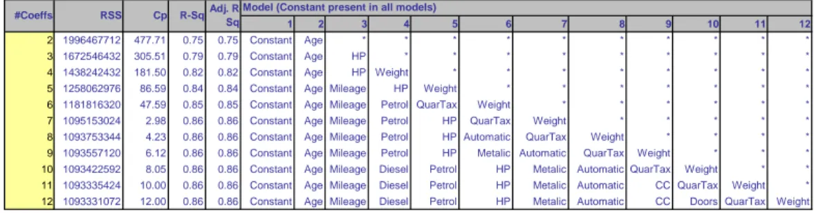
4.3 Variable Selection in Linear Regression . . . 59
4.3.1 The Need for Reducing the Number of Predictors . . . 59
4.3.2 How to reduce the number of predictors . . . 61
4.4 Exercises . . . 65
5 Logistic Regression 71 5.1 Example: Acceptance of Personal Loan . . . 72
5.1.1 Data preprocessing . . . 73
5.2 Why is Linear Regression Inappropriate for a Categorical Response? . . . 73
5.3 The Logistic Regression Model . . . 75
5.3.1 Estimating the Logistic Model From Data: Computing Parameter Estimates 79 5.3.2 Interpreting Results in Terms of Odds . . . 81
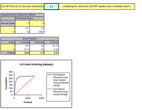
5.4 Evaluating Classification Performance . . . 82
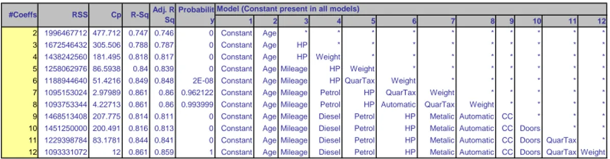
5.4.1 Variable Selection . . . 84
5.5 Evaluating Goodness of Fit . . . 85
5.6 Example of Complete Analysis: Predicting Delayed Flights . . . 86
5.7 Exercises . . . 94
5.8 Appendix: Logistic Regression for more than 2 groups . . . 97
5.8.1 Ordinal Groups . . . 97
5.8.2 Nominal Groups . . . 98
6 Neural Nets 101 6.1 The Neuron (a Mathematical Model) . . . 101
6.2 The Multilayer Neural Networks . . . 102
6.2.1 Single Layer Networks . . . 102
6.2.2 Multilayer Neural Networks . . . 104
6.3 Example 1: A Tiny Data Set . . . 105
6.4 Example 2: Accident Data . . . 106
6.5 The Backward Propagation Algorithm - Classification . . . 108
6.5.1 Forward Pass - Computation of Outputs of all the Neurons in the Network. . 108
CONTENTS iii
6.6 Adjustment for Prediction . . . 109
6.7 Multiple Local Optima and Epochs . . . 110
6.8 Overfitting and the choice of training epochs . . . 110
6.9 Adaptive Selection of Architecture . . . 110
6.10 Successful Applications . . . 111
7 Classification and Regression Trees 113 7.1 Classification Trees . . . 113
7.2 Recursive Partitioning . . . 113
7.3 Example 1 - Riding Mowers . . . 114
7.3.1 Measures of Impurity . . . 116
7.4 Evaluating the performance of a Classification tree . . . 120
7.5 Avoiding Overfitting . . . 121
7.5.1 Stopping tree growth: CHAID . . . 124
7.5.2 Pruning the tree . . . 125
7.6 Classification Rules from Trees . . . 129
7.7 Regression Trees . . . 129
7.7.1 Prediction . . . 132
7.7.2 Measuring impurity . . . 132
7.7.3 Evaluating performance . . . 132
7.8 Extensions and Conclusions . . . 132
7.9 Exercises . . . 133
8 Discriminant Analysis 137 8.1 Example 1 - Riding Mowers . . . 137
8.2 Example 2 - Personal Loan Acceptance . . . 138
8.3 The Distance of an Observation from a Group . . . 139
8.4 Fisher’s Linear Classification Functions . . . 141
8.5 Classification Performance of Discriminant Analysis . . . 145
8.6 Prior Probabilities . . . 146
8.7 Unequal Misclassification Costs . . . 146
8.8 Classifying More Than Two Groups . . . 147
9 Other Supervised Learning Techniques 153 9.1 K-Nearest neighbor . . . 153
9.1.1 The K-NN Procedure . . . 154
9.1.2 Example 1 - Riding Mowers . . . 154
9.1.3 K-Nearest Neighbor Prediction . . . 156
9.1.4 Shortcomings of k-NN algorithms . . . 156
9.2 Naive Bayes . . . 157
9.2.1 Bayes Theorem . . . 157
9.2.3 Simplify - assume independence . . . 158
9.2.4 Example 1 - Saris . . . 159
10 Affinity Analysis - Association Rules 163 10.1 Discovering Association Rules in Transaction Databases . . . 163
10.2 Support and Confidence . . . 163
10.3 Data Format . . . 165
10.4 Example 1 - Synthetic Data . . . 166
10.5 The Apriori Algorithm . . . 168
10.6 Example 2 - Applying and Interpreting Association Rules . . . 169
11 Data Exploration and Dimension Reduction 175 11.1 Practical Considerations . . . 175
11.2 Correlation Analysis . . . 175
11.3 Reducing the number of categories in categorical variables . . . 176
11.4 Principal Components Analysis . . . 176
11.4.1 Example: Breakfast Cereals . . . 176
11.4.2 The Principal Components . . . 181
11.4.3 Normalizing the Data . . . 181
11.4.4 Using the principal components for classification and prediction . . . 183
11.5 Exercises . . . 184
12 Cluster Analysis 187 12.1 What is Cluster Analysis? . . . 187
12.2 Example 1 - Public Utilities Data . . . 188
12.3 Hierarchical Methods . . . 190
12.3.1 Nearest neighbor (Single linkage) . . . 190
12.3.2 Farthest neighbor (Complete linkage) . . . 191
12.3.3 Group average (Average linkage) . . . 191
12.4 Optimization and thek-means algorithm . . . 193
12.5 Similarity Measures . . . 196
12.6 Other distance measures . . . 197
13 Cases 199 13.1 Charles Book Club . . . 199
13.2 German Credit . . . 207
13.3 Textile Cooperatives . . . 213
13.4 Tayko Software Cataloger . . . 216
13.5 IMRB : Segmenting Consumers of Bath Soap . . . 221
13.6 Direct Mail Fundraising For a Charity . . . 225
Chapter 1
Introduction
1.1
Who is This Book For?
This book arose out of a data mining course at MIT’s Sloan School of Management. Preparation for the course revealed that there are a number of excellent books on the business context of data mining, but their coverage of the statistical and machine-learning algorithms that underlie data mining is not sufficiently detailed to provide a practical guide if the instructor’s goal is to equip students with the skills and tools to implement those algorithms. On the other hand, there are also a number of more technical books about data mining algorithms, but these are aimed at the statistical researcher, or more advanced graduate student, and do not provide the case-oriented business focus that is successful in teaching business students.
Hence, this book is intended for the business student (and practitioner) of data mining tech-niques, and its goal is threefold:
1. To provide both a theoretical and practical understanding of the key methods of classification, prediction, reduction and exploration that are at the heart of data mining;
2. To provide a business decision-making context for these methods;
3. Using real business cases, to illustrate the application and interpretation of these methods.
An important feature of this book is the use of Excel, an environment familiar to business analysts. All required data mining algorithms (plus illustrative data sets) are provided in an Excel add-in, XLMiner. The presentation of the cases is structured so that the reader can follow along and implement the algorithms on his or her own with a very low learning curve.
While the genesis for this book lay in the need for a case-oriented guide to teaching data-mining, analysts and consultants who are considering applying data mining techniques in contexts where they are not currently in use will also find this a useful, practical guide.
1.2
What is Data Mining?
The field of data mining is still relatively new, and in a state of evolution. The first International Conference on Knowledge Discovery and Data Mining (“KDD”) was held in 1995, and there are a variety of definitions of data mining.
A concise definition that captures the essence of data mining is:
“Extracting useful information from large data sets” (Hand, et al: 2001). A slightly longer version is:
“Data mining is the process of exploration and analysis, by automatic or semi-automatic means, of large quantities of data in order to discover meaningful patterns and rules.” (Berry and Linoff: 1997 and 2000)
Berry and Linoff later had cause to regret the 1997 reference to “automatic and semi-automatic means,” feeling it shortchanged the role of data exploration and analysis.
Another definition comes from the Gartner Group, the information technology research firm (from their web site, Jan. 2004):
“Data mining is the process of discovering meaningful new correlations, patterns and trends by sifting through large amounts of data stored in repositories, using pattern recognition technologies as well as statistical and mathematical techniques.”
A summary of the variety of methods encompassed in the term “data mining” follows below (“Core Ideas”).
1.3
Where is Data Mining Used?
Data mining is used in a variety of fields and applications. The military might use data mining to learn what roles various factors play in the accuracy of bombs. Intelligence agencies might use it to determine which of a huge quantity of intercepted communications are of interest. Security specialists might use these methods to determine whether a packet of network data constitutes a threat. Medical researchers might use them to predict the likelihood of a cancer relapse.
Although data mining methods and tools have general applicability, in this book most examples are chosen from the business world. Some common business questions one might address through data mining methods include:
1. From a large list of prospective customers, which are most likely to respond? We could use classification techniques (logistic regression, classification trees or other methods) to identify those individuals whose demographic and other data most closely matches that of our best existing customers. Similarly, we can use prediction techniques to forecast how much individual prospects will spend.
2. Which customers are most likely to commit fraud (or might already have committed it)? We can use classification methods to identify (say) medical reimbursement applications that have a higher probability of involving fraud, and give them greater attention.
1.4 The Origins of Data Mining 3 3. Which loan applicants are likely to default? We might use classification techniques to identify
them (or logistic regression to assign a “probability of default” value).
4. Which customers are more likely to abandon a subscription service (telephone, magazine, etc.)? Again, we might use classification techniques to identify them (or logistic regression to assign a “probability of leaving” value). In this way, discounts or other enticements might be proffered selectively where they are most needed.
1.4
The Origins of Data Mining
Data mining stands at the confluence of the fields of statistics and machine learning (also known as artificial intelligence). A variety of techniques for exploring data and building models have been around for a long time in the world of statistics - linear regression, logistic regression, discriminant analysis and principal components analysis, for example. But the core tenets of classical statistics-computing is difficult and data are scarce - do not apply in data mining applications where both data and computing power are plentiful.
This gives rise to Daryl Pregibon’s description of data mining as “statistics at scale and speed.” A useful extension of this is “statistics at scale, speed, and simplicity.” Simplicity in this case refers not to simplicity of algorithms, but rather to simplicity in the logic of inference. Due to the scarcity of data in the classical statistical setting, the same sample is used to make an estimate, and also to determine how reliable that estimate might be. As a result, the logic of the confidence intervals and hypothesis tests used for inference is elusive for many, and their limitations are not well appreciated. By contrast, the data mining paradigm of fitting a model with one sample and assessing its performance with another sample is easily understood.
Computer science has brought us “machine learning” techniques, such as trees and neural net-works, that rely on computational intensity and are less structured than classical statistical models. In addition, the growing field of database management is also part of the picture.
The emphasis that classical statistics places on inference (determining whether a pattern or interesting result might have happened by chance) is missing in data mining. In comparison to statistics, data mining deals with large data sets in open-ended fashion, making it impossible to put the strict limits around the question being addressed that inference would require.
As a result, the general approach to data mining is vulnerable to the danger of “overfitting,” where a model is fit so closely to the available sample of data that it describes not merely structural characteristics of the data, but random peculiarities as well. In engineering terms, the model is fitting the noise, not just the signal.
1.5
Terminology and Notation
Because of the hybrid parentry of data mining, its practitioners often use multiple terms to refer to the same thing. For example, in the machine learning (artificial intelligence) field, the variable
being predicted is the output variable or the target variable. To a statistician, it is the dependent variable. Here is a summary of terms used:
“Algorithm” refers to a specific procedure used to implement a particular data mining technique-classification tree, discriminant analysis, etc.
“Attribute” is also called a “feature,” “variable,” or, from a database perspective, a “field.” “Case” is a set of measurements for one entity - e.g. the height, weight, age, etc. of one person; also called “record,” “pattern” or “row”. (each row typically represents a record, each column a variable)
“Confidence” has a specific meaning in association rules of the type “If A and B are purchased, C is also purchased.” Confidence is the conditional probability that C will be purchased, IF A and B are purchased.
“Confidence” also has a broader meaning in statistics (“confidence interval”), concerning the degree of error in an estimate that results from selecting one sample as opposed to another.
“Dependent variable” is the variable being predicted in supervised learning; also called “output variable,” “target variable” or “outcome variable.”
“Estimation” means the prediction of the value of a continuous output variable; also called “prediction.”
“Feature” is also called an “attribute,” “variable,” or, from a database perspective, a “field.” “Input variable” is a variable doing the predicting in supervised learning; also called “indepen-dent variable,” “predictor.”
“Model” refers to an algorithm as applied to a data set, complete with its settings (many of the algorithms have parameters which the user can adjust).
“Outcome variable” is the variable being predicted in supervised learning; also called “dependent variable,” “target variable” or “output variable.”
“Output variable” is the variable being predicted in supervised learning; also called “dependent variable,” “target variable” or “outcome variable.”
“P(A|B)” is read as “the probability thatAwill occur, given thatB has occurred.”
“Pattern” is a set of measurements for one entity - e.g. the height, weight, age, etc. of one person; also called “record,” “case” or “row”. (each row typically represents a record, each column a variable)
“Prediction” means the prediction of the value of a continuous output variable; also called “estimation.”
“Record” is a set of measurements for one entity - e.g. the height, weight, age, etc. of one person; also called “case,” “pattern” or “row”. (each row typically represents a record, each column a variable)
“Score” refers to a predicted value or class. “Scoring new data” means to use a model developed with training data to predict output values in new data.
“Supervised learning” refers to the process of providing an algorithm (logistic regression, re-gression tree, etc.) with records in which an output variable of interest is known and the algorithm “learns” how to predict this value with new records where the output is unknown.
1.6 Organization of Data Sets 5 “Test data” refers to that portion of the data used only at the end of the model building and selection process to assess how well the final model might perform on additional data.
“Training data” refers to that portion of data used to fit a model.
“Unsupervised learning” refers to analysis in which one attempts to learn something about the data other than predicting an output value of interest (whether it falls into clusters, for example).
“Validation data” refers to that portion of the data used to assess how well the model fits, to adjust some models, and to select the best model from among those that have been tried.
“Variable” is also called a “feature,” “attribute,” or, from a database perspective, a “field.”
1.6
Organization of Data Sets
Data sets are nearly always constructed and displayed so that variables are in columns, and records are in rows. In the example below (the Boston Housing data), the values of 14 variables are recorded for a number of census tracts. Each row represents a census tract - the first tract had a per capital crime rate (CRIM) of 0.02729, had 0 of its residential lots zoned for over 25,000 square feet (ZN), etc. In supervised learning situations, one of these variables will be the outcome variable, typically listed at the end or the beginning (in this case it is median value, MEDV, at the end).
1.7
Factors Responsible for the Rapid Growth of Data
Min-ing
Perhaps the most important factor propelling the growth of data mining is the growth of data. The mass retailer Walmart in 2003 captured 20 million transactions per day in a 10-terabyte database. In 1950, the largest companies had only enough data to occupy, in electronic form, several dozen megabytes (a terabyte is 1,000,000 megabytes).
The growth of data themselves is driven not simply by an expanding economy and knowledge base, but by the decreasing cost and increasing availability of automatic data capture mechanisms. Not only are more events being recorded, but more information per event is captured. Scannable bar codes, point of sale (POS) devices, mouse click trails, and global positioning satellite (GPS) data are examples.
The growth of the internet has created a vast new arena for information generation. Many of the same actions that people undertake in retail shopping, exploring a library or catalog shopping have close analogs on the internet, and all can now be measured in the most minute detail.
In marketing, a shift in focus from products and services to a focus on the customer and his or her needs has created a demand for detailed data on customers.
The operational databases used to record individual transactions in support of routine business activity can handle simple queries, but are not adequate for more complex and aggregate analysis. Data from these operational databases are therefore extracted, transformed and exported to adata
warehouse - a large integrated data storage facility that ties together the decision support systems
of an enterprise. Smaller data marts devoted to a single subject may also be part of the system. They may include data from external sources (e.g. credit rating data).
Many of the exploratory and analytical techniques used in data mining would not be possible without today’s computational power. The constantly declining cost of data storage and retrieval has made it possible to build the facilities required to store and make available vast amounts of data. In short, the rapid and continuing improvement in computing capacity is an essential enabler of the growth of data mining.
Chapter 2
Overview of the Data Mining
Process
2.1
Core Ideas in Data Mining
2.1.1
Classification
Classification is perhaps the most basic form of data analysis. The recipient of an offer might respond or not respond. An applicant for a loan might repay on time, repay late or declare bankruptcy. A credit card transaction might be normal or fraudulent. A packet of data traveling on a network might be benign or threatening. A bus in a fleet might be available for service or unavailable. The victim of an illness might be recovered, still ill, or deceased.
A common task in data mining is to examine data where the classification is unknown or will occur in the future, with the goal of predicting what that classification is or will be. Similar data where the classification is known are used to develop rules, which are then applied to the data with the unknown classification.
2.1.2
Prediction
Prediction is similar to classification, except we are trying to predict the value of a variable (e.g. amount of purchase), rather than a class (e.g. purchaser or nonpurchaser).
Of course, in classification we are trying to predict a class, but the term “prediction” in this book refers to the prediction of the value of a continuous variable. (Sometimes in the data mining literature, the term “estimation” is used to refer to the prediction of the value of a continuous variable, and “prediction” may be used for both continuous and categorical data.)
2.1.3
Affinity Analysis
Large databases of customer transactions lend themselves naturally to the analysis of associations among items purchased, or “what goes with what.” “Association rules” can then be used in a variety of ways. For example, grocery stores might use such information after a customer’s purchases have
all been scanned to print discount coupons, where the items being discounted are determined by mapping the customers purchases onto the association rules.
2.1.4
Data Reduction
Sensible data analysis often requires distillation of complex data into simpler data. Rather than dealing with thousands of product types, an analyst might wish to group them into a smaller number of groups. This process of consolidating a large number of variables (or cases) into a smaller set is termed data reduction.
2.1.5
Data Exploration
Unless our data project is very narrowly focused on answering a specific question determined in advance (in which case it has drifted more into the realm of statistical analysis than of data mining), an essential part of the job is to review and examine the data to see what messages it holds, much as a detective might survey a crime scene. Here, full understanding of the data may require a reduction in its scale or dimension to let us to see the forest without getting lost in the trees. Similar variables (i.e. variables that supply similar information) might be aggregated into a single variable incorporating all the similar variables. Analogously, cluster analysis might be used to aggregate records together into groups of similar records.
2.1.6
Data Visualization
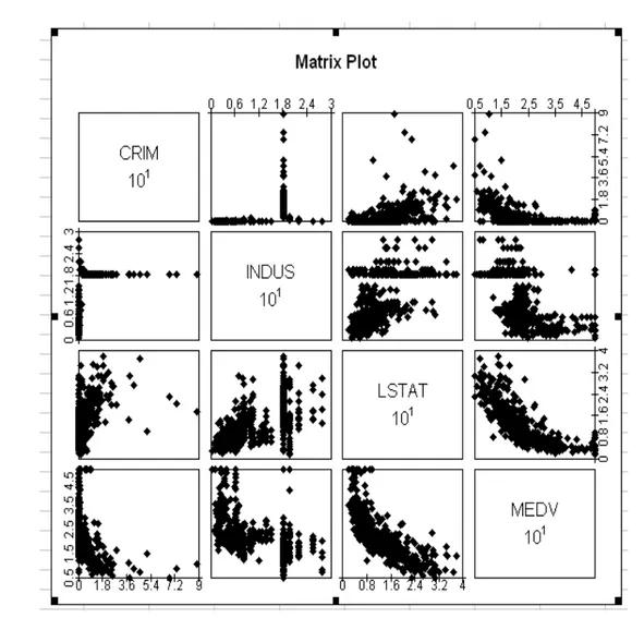
Another technique for exploring data to see what information they hold is graphical analysis. For example, combining all possible scatter plots of one variable against another on a single page allows us to quickly visualize relationships among variables.
The Boston Housing data is used to illustrate this. In this data set, each row is a city neighbor-hood (census tract, actually) and each column is a variable (crime rate, pupil/teacher ratio, etc.). The outcome variable of interest is the median value of a housing unit in the neighborhood. Figure 2.1 takes four variables from this data set and plots them against each other in a series of two-way scatterplots. In the lower left, for example, the crime rate (CRIM) is plotted on the x-axis and the median value (MEDV) on the y-axis. In the upper right, the same two variables are plotted on op-posite axes. From the plots in the lower right quadrant, we see that, unsurprisingly, the more lower economic status residents a neighborhood has, the lower the median house value. From the upper right and lower left corners we see (again, unsurprisingly) that higher crime rates are associated with lower median values. An interesting result can be seen in the upper left quadrant. All the very high crime rates seem to be associated with a specific, mid-range value of INDUS (proportion of non-retail businesses per neighborhood). That a specific, middling level of INDUS is really associated with high crime rates seems dubious. A closer examination of the data reveals that each specific value of INDUS is shared by a number of neighborhoods, indicating that INDUS is measured for a broader area than that of the census tract neighborhood. The high crime rate associated so markedly with a specific value of INDUS indicates that the few neighborhoods with extremely high crime rates fall mainly within one such broader area.
2.2 Supervised and Unsupervised Learning 9 .
Figure 2.1 : Matrix scatterplot for four variables from the Boston Housing data.
2.2
Supervised and Unsupervised Learning
A fundamental distinction among data mining techniques is between supervised methods and unsu-pervised methods.
“Supervised learning” algorithms are those used in classification and prediction. We must have data available in which the value of the outcome of interest (e.g. purchase or no purchase) is known. These “training data” are the data from which the classification or prediction algorithm “learns,” or is “trained,” about the relationship between predictor variables and the outcome variable. Once the algorithm has learned from the training data, it is then applied to another sample of data (the “validation data”) where the outcome is known, to see how well it does in comparison to other models. If many different models are being tried out, it is prudent to save a third sample of known outcomes (the “test data”) to use with the final, selected model to predict how well it will do. The
model can then be used to classify or predict the outcome variable of interest in new cases where the outcome is unknown.
Simple linear regression analysis is an example of supervised learning (though rarely called that in the introductory statistics course where you likely first encountered it). The Y variable is the (known) outcome variable. A regression line is drawn to minimize the sum of squared deviations between the actual Y values and the values predicted by this line. The regression line can now be used to predict Y values for new values ofX for which we do not know theY value.
Unsupervised learning algorithms are those used where there is no outcome variable to predict or classify. Hence, there is no “learning” from cases where such an outcome variable is known. Affinity analysis, data reduction methods and clustering techniques are all unsupervised learning methods.
2.3
The Steps In Data Mining
This book focuses on understanding and using data mining algorithms (steps 4-7 below). However, some of the most serious errors in data analysis result from a poor understanding of the problem - an understanding that must be developed well before we get into the details of algorithms to be used. Here is a list of the steps to be taken in a typical data mining effort:
1. Develop an understanding of the purpose of the data mining project (if it is a one-shot effort to answer a question or questions) or application (if it is an ongoing procedure).
2. Obtain the data set to be used in the analysis. This often involves random sampling from a large database to capture records to be used in an analysis. It may also involve pulling together data from different databases. The databases could be internal (e.g. past purchases made by customers) or external (credit ratings). While data mining deals with very large databases, usually the analysis to be done requires only thousands or tens of thousands of records. 3. Explore, clean, and preprocess the data. This involves verifying that the data are in reasonable
condition. How should missing data be handled? Are the values in a reasonable range, given what you would expect for each variable? Are there obvious “outliers?” The data are reviewed graphically - for example, a matrix of scatterplots showing the relationship of each variable with each other variable. We also need to ensure consistency in the definitions of fields, units of measurement, time periods, etc.
4. Reduce the data, if necessary, and (where supervised training is involved) separate it into train-ing, validation and test data sets. This can involve operations such as eliminating unneeded variables, transforming variables (for example, turning “money spent” into “spent>$100” vs. “spent<= $100”), and creating new variables (for example, a variable that records whether at least one of several products was purchased). Make sure you know what each variable means, and whether it is sensible to include it in the model.
5. Determine the data mining task (classification, prediction, clustering, etc.). This involves translating the general question or problem of step 1 into a more specific statistical question.
2.4 SEMMA 11 6. Choose the data mining techniques to be used (regression, neural nets, Ward’s method of
hierarchical clustering, etc.).
7. Use algorithms to perform the task. This is typically an iterative process - trying multiple variants, and often using multiple variants of the same algorithm (choosing different variables or settings within the algorithm). Where appropriate, feedback from the algorithm’s performance on validation data is used to refine the settings.
8. Interpret the results of the algorithms. This involves making a choice as to the best algorithm to deploy, and, where possible, testing our final choice on the test data to get an idea how well it will perform. (Recall that each algorithm may also be tested on the validation data for tuning purposes; in this way the validation data becomes a part of the fitting process and is likely to underestimate the error in the deployment of the model that is finally chosen.) 9. Deploy the model. This involves integrating the model into operational systems and running
it on real records to produce decisions or actions. For example, the model might be applied to a purchased list of possible customers, and the action might be “include in the mailing if the predicted amount of purchase is>$10.”
2.4
SEMMA
The above steps encompass the steps in SEMMA, a methodology developed by SAS: Sample from data sets, partition into training, validation and test data sets
Explore data set statistically and graphically Modify: transform variables, impute missing values
Model: fit predictive models, e.g. regression, tree, collaborative filtering Assess: compare models using validation data set
SPSS-Clementine also has a similar methodology, termed CRISP-DM (CRoss-Industry Standard Process for Data Mining).
2.5
Preliminary Steps
2.5.1
Sampling from a Database
Quite often, we will want to do our data mining analysis on less than the total number of records that are available. Data mining algorithms will have varying limitations on what they can handle in terms of the numbers of records and variables, limitations that may be specific to computing power and capacity as well as software limitations. Even within those limits, many algorithms will execute faster with smaller data sets.
From a statistical perspective, accurate models can often be built with as few as several hundred records (see below). Hence, often we will want to sample a subset of records for model building.
2.5.2
Oversampling Rare Events
If the event we are interested in is rare, however, (e.g. customers purchasing a product in response to a mailing), sampling a subset of records may yield so few events (e.g. purchases) that we have little information on them. We would end up with lots of data on non-purchasers, but little on which to base a model that distinguishes purchasers from non-purchasers. In such cases, we would want our sampling procedure to over-weight the purchasers relative to the non-purchasers so that our sample would end up with a healthy complement of purchasers. This issue arises mainly in classification problems because those are the types of problems in which an overwhelming number of 0’s is likely to be encountered in the response variable. While the same principle could be extended to prediction, any prediction problem in which most responses are 0 is likely to raise the question of what distinguishes responses from non-responses (i.e. a classification question). (For convenience below we speak of responders and non-responders, as to a promotional offer, but we are really referring to any binary - 0/1 - outcome situation.)
Assuring an adequate number of responder or “success” cases to train the model is just part of the picture. A more important factor is the costs of misclassification. Whenever the response rate is extremely low, we are likely to attach more importance to identifying a responder than identifying a non-responder. In direct response advertising (whether by traditional mail or via the internet), we may encounter only one or two responders for every hundred records - the value of finding such a customer far outweighs the costs of reaching him or her. In trying to identify fraudulent transactions, or customers unlikely to repay debt, the costs of failing to find the fraud or the non-paying customer likely exceed the cost of more detailed review of a transaction or customer who turns out to be okay. If the costs of failing to locate responders were comparable to the costs of misidentifying re-sponders as non-rere-sponders, our models would usually be at their best if they identify everyone (or almost everyone, if it is easy to pick off a few responders without catching many non-responders) as a non-responder. In such a case, the misclassification rate is very low - equal to the rate of responders - but the model is of no value.
More generally, we want to train our model with the asymmetric costs in mind, so that the algorithm will catch the more valuable responders, probably at the cost of “catching,” and misclas-sifying, more non-responders as responders than would be the case if we assume equal costs. This subject is discussed in detail in the next chapter.
2.5.3
Pre-processing and Cleaning the Data
2.5.3.1 Types of Variables
There are several ways of classifying variables. Variables can be numeric or text (character). They can be continuous (able to assume any real numeric value, usually in a given range), integer (assum-ing only integer values), or categorical (assum(assum-ing one of a limited number of values). Categorical variables can be either numeric (1,2,3) or text (payments current, payments not current, bankrupt). Categorical variables can also be unordered (North America, Europe, Asia) or ordered (high value, low value, nil value).
2.5 Preliminary Steps 13 take continuous variables, with the exception of Nave Bayes classifier, which deals exclusively with categorical variables. Sometimes, it is desirable to convert continuous variables to categorical ones. This is done most typically in the case of outcome variables, where the numerical variable is mapped to a decision (e.g. credit scores above a certain level mean “grant credit,” a medical test result above a certain level means “start treatment.”) XLMiner has a facility for this.
2.5.3.2 Handling Categorical Variables
Categorical variables can also be handled by most routines, but often require special handling. If the categorical variable is ordered (for example, age category, degree of creditworthiness, etc.), then we can often use it as is, as if it were a continuous variable. The smaller the number of categories, and the less they represent equal increments of value, the more problematic this procedure is, but it often works well enough.
Unordered categorical variables, however, cannot be used as is. They must be decomposed into a series of dummy binary variables. For example, a single variable in that can have possible values of “student,” “unemployed,” “employed,” or “retired” would be split into four separate variables:
Student - yes/no Unemployed - yes/no Employed - yes/no Retired - yes/no
Note that only three of the variables need to be used - if the values of three are known, the fourth is also known. For example, given that these four values are the only possible ones, we can know that if a person is neither student, unemployed, nor employed, he or she must be retired. In some routines (e.g. regression and logistic regression), you should not use all four variables - the redundant information will cause the algorithm to fail.
XLMiner has a utility to convert categorical variables to binary dummies. 2.5.3.3 Variable Selection
More is not necessarily better when it comes to selecting variables for a model. Other things being equal, parsimony, or compactness, is a desirable feature in a model.
For one thing, the more variables we include, the greater the number of records we will need to assess relationships among the variables. 15 records may suffice to give us a rough idea of the relationship betweenY and a single dependent variableX. If we now want information about the relationship between Y and fifteen dependent variables X1· · ·X15, fifteen dependent variables will
not be enough (each estimated relationship would have an average of only one record’s worth of information, making the estimate very unreliable).
2.5.3.4 Overfitting
For another thing, the more variables we include, the greater the risk of overfitting the data. What is overfitting?
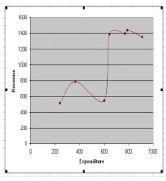
Consider the following hypothetical data about advertising expenditures in one time period, and sales in a subsequent time period:
Advertising Sales 239 514 364 789 602 550 644 1386 770 1394 789 1440 911 1354
Figure 2.2 : X-Y scatterplot for advertising and sales data
We could connect up these lines with a smooth and very complex function, one that explains all these data points perfectly and leaves no error (residuals).
2.5 Preliminary Steps 15 .
Figure 2.3 : X-Y scatterplot, smoothed
However, we can see that such a curve is unlikely to be that accurate, or even useful, in predicting future sales on the basis of advertising expenditures.
A basic purpose of building a model is to describe relationships among variables in such a way that this description will do a good job of predicting future outcome (dependent) values on the basis of future predictor (independent) values. Of course, we want the model to do a good job of describing the data we have, but we are more interested in its performance with data to come.
In the above example, a simple straight line might do a better job of predicting future sales on the basis of advertising than the complex function does.
In this example, we devised a complex function that fit the data perfectly, and in doing so over-reached. We certainly ended up “explaining” some variation in the data that was nothing more than chance variation. We have mislabeled the noise in the data as if it were a signal.
Similarly, we can add predictors to a model to sharpen its performance with the data at hand. Consider a database of 100 individuals, half of whom have contributed to a charitable cause. In-formation about income, family size, and zip code might do a fair job of predicting whether or not someone is a contributor. If we keep adding additional predictors, we can improve the performance of the model with the data at hand and reduce the misclassification error to a negligible level. However, this low error rate is misleading, because it likely includes spurious “explanations.”
For example, one of the variables might be height. We have no basis in theory to suppose that tall people might contribute more or less to charity, but if there are several tall people in our sample and they just happened to contribute heavily to charity, our model might include a term for height
-the taller you are, -the more you will contribute. Of course, when -the model is applied to additional data, it is likely that this will not turn out to be a good predictor.
If the data set is not much larger than the number of predictor variables, then it is very likely that a spurious relationship like this will creep into the model. Continuing with our charity example, with a small sample just a few of whom are tall, whatever the contribution level of tall people may be, the computer is tempted to attribute it to their being tall. If the data set is very large relative to the number of predictors, this is less likely. In such a case, each predictor must help predict the outcome for a large number of cases, so the job it does is much less dependent on just a few cases, which might be flukes.
Overfitting can also result from the application of many different models, from which the best performing is selected (more about this below).
2.5.3.5 How Many Variables and How Much Data?
Statisticians could give us procedures to learn with some precision how many records we would need to achieve a given degree of reliability with a given data set and a given model. Data miners’ needs are usually not so precise, so we can often get by with rough rules of thumb. A good rule of thumb is to have ten records for every predictor variable. Another, used by Delmater and Hancock for classification procedures (2001, p. 68) is to have at least 6*M*N records, where
M = number of outcome classes, and N = number of variables
Even when we have an ample supply of data, there are good reasons to pay close attention to the variables that are included in a model. Someone with domain knowledge (i.e. knowledge of the business process and the data) should be consulted - knowledge of what the variables represent can often help build a good model and avoid errors.
For example, “shipping paid” might be an excellent predictor of “amount spent,” but it is not a helpful one. It will not give us any information about what distinguishes high-paying from low-paying customers that can be put to use with future prospects, because we will not have the “shipping paid” information for prospects that have not yet bought anything.
In general, compactness or parsimony is a desirable feature in a model. A matrix of X-Y plots can be useful in variable selection. In such a matrix, we can see at a glance x-y plots for all variable combinations. A straight line would be an indication that one variable is exactly correlated with another. Typically, we would want to include only one of them in our model. The idea is to weed out irrelevant and redundant variables from our model.
2.5.3.6 Outliers
The more data we are dealing with, the greater the chance of encountering erroneous values resulting from measurement error, data entry error, or the like. If the erroneous value is in the same range as the rest of the data, it may be harmless. If it is well outside the range of the rest of the data (a misplaced decimal, for example), it may have substantial effect on some of the data mining procedures we plan to use.
2.5 Preliminary Steps 17 Values that lie far away from the bulk of the data are called outliers. The term “far away” is deliberately left vague because what is or is not called an outlier is basically an arbitrary decision. Analysts use rules of thumb like “anything over 3 standard deviations away from the mean is an outlier,” but no statistical rule can tell us whether such an outlier is the result of an error. In this statistical sense, an outlier is not necessarily an invalid data point, it is just a distant data point.
The purpose of identifying outliers is usually to call attention to values that need further review. We might come up with an explanation looking at the data - in the case of a misplaced decimal, this is likely. We might have no explanation, but know that the value is wrong - a temperature of 178 degrees F for a sick person. Or, we might conclude that the value is within the realm of possibility and leave it alone. All these are judgments best made by someone with “domain” knowledge. (Domain knowledge is knowledge of the particular application being considered – direct mail, mortgage finance, etc., as opposed to technical knowledge of statistical or data mining procedures.) Statistical procedures can do little beyond identifying the record as something that needs review.
If manual review is feasible, some outliers may be identified and corrected. In any case, if the number of records with outliers is very small, they might be treated as missing data.
How do we inspect for outliers? One technique in Excel is to sort the records by the first column, then review the data for very large or very small values in that column. Then repeat for each successive column. For a more automated approach that considers each record as a unit, clustering techniques could be used to identify clusters of one or a few records that are distant from others. Those records could then be examined.
2.5.3.7 Missing Values
Typically, some records will contain missing values. If the number of records with missing values is small, those records might be omitted.
However, if we have a large number of variables, even a small proportion of missing values can affect a lot of records. Even with only 30 variables, if only 5% of the values are missing (spread randomly and independently among cases and variables), then almost 80% of the records would have to be omitted from the analysis. (The chance that a given record would escape having a missing value is 0.9530= 0.215.)
An alternative to omitting records with missing values is to replace the missing value with an imputed value, based on the other values for that variable across all records. For example, if, among 30 variables, household income is missing for a particular record, we might substitute instead the mean household income across all records.
Doing so does not, of course, add any information about how household income affects the outcome variable. It merely allows us to proceed with the analysis and not lose the information contained in this record for the other 29 variables. Note that using such a technique will understate the variability in a data set. However, since we can assess variability, and indeed the performance of our data mining technique, using the validation data, this need not present a major problem.
2.5.3.8 Normalizing (Standardizing) the Data
Some algorithms require that the data be normalized before the algorithm can be effectively imple-mented. To normalize the data, we subtract the mean from each value, and divide by the standard deviation of the resulting deviations from the mean. In effect, we are expressing each value as “number of standard deviations away from the mean.”
To consider why this might be necessary, consider the case of clustering. Clustering typically involves calculating a distance measure that reflects how far each record is from a cluster center, or from other records. With multiple variables, different units will be used - days, dollars, counts, etc. If the dollars are in the thousands and everything else is in the 10’s, the dollar variable will come to dominate the distance measure. Moreover, changing units from (say) days to hours or months could completely alter the outcome.
Data mining software, including XLMiner, typically has an option that normalizes the data in those algorithms where it may be required. It is an option, rather than an automatic feature of such algorithms, because there are situations where we want the different variables to contribute to the distance measure in proportion to their scale.
2.5.4
Use and Creation of Partitions
In supervised learning, a key question presents itself:
How well will our prediction or classification model perform when we apply it to new data? We are particularly interested in comparing the performance among various models, so we can choose the one we think will do the best when it is actually implemented.
At first glance, we might think it best to choose the model that did the best job of classifying or predicting the outcome variable of interest with the data at hand. However, when we use the same data to develop the model then assess its performance, we introduce bias.
This is because when we pick the model that does best with the data, this model’s superior performance comes from two sources:
• A superior model
• Chance aspects of the data that happen to match the chosen model better than other models. The latter is a particularly serious problem with techniques (such as trees and neural nets) that do not impose linear or other structure on the data, and thus end up overfitting it.
To address this problem, we simply divide (partition) our data and develop our model using only one of the partitions. After we have a model, we try it out on another partition and see how it does. We can measure how it does in several ways. In a classification model, we can count the proportion of held-back records that were misclassified. In a prediction model, we can measure the residuals (errors) between the predicted values and the actual values.
2.6 Building a Model ... 19 2.5.4.1 Training Partition
The training partition is typically the largest partition, and contains the data used to build the various models we are examining. The same training partition is generally used to develop multiple models.
2.5.4.2 Validation Partition
This partition (sometimes called the “test” partition) is used to assess the performance of each model, so that you can compare models and pick the best one. In some algorithms (e.g. classification and regression trees), the validation partition may be used in automated fashion to tune and improve the model.
2.5.4.3 Test Partition
This partition (sometimes called the “holdout” or “evaluation” partition) is used if we need to assess the performance of the chosen model with new data.
Why have both a validation and a test partition? When we use the validation data to assess multiple models and then pick the model that does best with the validation data, we again encounter another (lesser) facet of the overfitting problem – chance aspects of the validation data that happen to match the chosen model better than other models.
The random features of the validation data that enhance the apparent performance of the chosen model will not likely be present in new data to which the model is applied. Therefore, we may have overestimated the accuracy of our model. The more models we test, the more likely it is that one of them will be particularly effective in explaining the noise in the validation data. Applying the model to the test data, which it has not seen before, will provide an unbiased estimate of how well it will do with new data.
Sometimes (for example, when we are concerned mainly with finding the best model and less with exactly how well it will do), we might use only training and validation partitions.
The partitioning should be done randomly to avoid getting a biased partition. In XLMiner, the user can supply a variable (column) with a value “t” (training), “v” (validation) and “s” (test) assigned to each case (row). Note that with nearest neighbor algorithms the training data itself is the model – records in the validation and test partitions, and in new data, are compared to records in the training data to find the nearest neighbor(s). As k-nearest-neighbors is implemented in XLMiner and as discussed in this book, the use of two partitions is an essential part of the classification or prediction process, not merely a way to improve or assess it. Nonetheless, we can still interpret the error in the validation data in the same way we would interpret error from any other model.
XLMiner has a utility that can divide the data up into training, validation and test sets either randomly according to user-set proportions, or on the basis of a variable that denotes which partition a record is to belong to. It is possible (though cumbersome) to divide the data into more than 3 partitions by successive partitioning - e.g. divide the initial data into 3 partitions, then take one of those partitions and partition it further.
2.6
Building a Model - An Example with Linear Regression
Let’s go through the steps typical to many data mining tasks, using a familiar procedure - multiple linear regression. This will help us understand the overall process before we begin tackling new algorithms. We will illustrate the Excel procedure using XLMiner.
1. Purpose. Let’s assume that the purpose of our data mining project is to predict the median house value in small Boston area neighborhoods.
2. Obtain the data. We will use the Boston Housing data. The data set in question is small enough that we do not need to sample from it - we can use it in its entirety.
3. Explore, clean, and preprocess the data.
Let’s look first at the description of the variables (crime rate, number of rooms per dwelling, etc.) to be sure we understand them all. These descriptions are available on the “description” tab on the worksheet, as is a web source for the data set. They all seem fairly straightforward, but this is not always the case. Often variable names are cryptic and their descriptions may be unclear or missing.
This data set has 14 variables and a description of each variable is given in the table below.
CRIM Per capita crime rate by town
ZN Proportion of residential land zoned for lots over 25,000 sq.ft.
INDUS Proportion of non-retail business acres per town CHAS Charles River dummy variable (= 1 if tract
bounds river; 0 otherwise)
NOX Nitric oxides concentration (parts per 10 million) RM Average number of rooms per dwelling
AGE Proportion of owner-occupied units built prior to 1940 DIS Weighted distances to five Boston employment centers RAD Index of accessibility to radial highways
TAX Full-value property-tax rate per $10,000 PTRATIO Pupil-teacher ratio by town
B 1000(Bk - 0.63)2 where Bk is the proportion of blacks by town
LSTAT % Lower status of the population
2.6 Building a Model ... 21 The data themselves look like this:
Figure 2.4
It is useful to pause and think about what the variables mean, and whether they should be included in the model. Consider the variable TAX. At first glance, we consider that tax on a home is usually a function of its assessed value, so there is some circularity in the model - we want to predict a home’s value using TAX as a predictor, yet TAX itself is determined by a home’s value. TAX might be a very good predictor of home value in a numerical sense, but would it be useful if we wanted to apply our model to homes whose assessed value might not be known? Reflect, though, that the TAX variable, like all the variables, pertains to the average in a neighborhood, not to individual homes. While the purpose of our inquiry has not been spelled out, it is possible that at some stage we might want to apply a model to individual homes and, in such a case, the neighborhood TAX value would be a useful predictor. So, we will keep TAX in the analysis for now.
In addition to these variables, the data set also contains an additional variable, CATMEDV, which has been created by categorizing median value (MEDV) into two categories – high and low. The variable CATMEDV is actually a categorical variable created from MEDV. If MEDV >=$30,000, CATV = 1. If MEDV<=$30,000, CATV = 0. If we were trying to categorize the cases into high and low median values, we would use CAT MEDV instead of MEDV. As it is, we do not need CAT MEDV so we will leave it out of the analysis.
There are a couple of aspects of MEDV− the median house value−that bear noting. For one thing, it is quite low, since it dates from the 1970’s. For another, there are a lot of 50’s, the top value. It could be that median values above $50,000 were recorded as $50,000. We are left with 13 independent (predictor) variables, which can all be used.
It is also useful to check for outliers that might be errors. For example, suppose the RM (# of rooms) column looked like this, after sorting the data in descending order based on rooms:
.
Figure 2.5
We can tell right away that the 79.29 is in error - no neighborhood is going to have houses that have an average of 79 rooms. All other values are between 3 and 9. Probably, the decimal was misplaced and the value should be 7.929. (This hypothetical error is not present in the data set supplied with XLMiner.)
4. Reduce the data and partition it into training, validation and test partitions. Our data set has only 13 variables, so data reduction is not required. If we had many more variables, at this stage we might want to apply a variable reduction technique such as Principal Components Analysis to consolidate multiple similar variables into a smaller number of variables. Our task is to predict the median house value, and then assess how well that prediction does. We will partition the data into a training set to build the model, and a validation set to see how well the model does. This technique is part of the “supervised learning” process in classification and prediction problems. These are problems in which we know the class or value of the outcome variable for some data, and we want to use that data in developing a model that can then be applied to other data where that value is unknown.
2.6 Building a Model ... 23 .
Figure 2.6
Here we specify which data range is to be partitioned, and which variables are to be included in the partitioned data set.
The partitioning can be handled in one of two ways:
a) The data set can have a partition variable that governs the division into training and validation partitions (e.g. 1 = training, 2 = validation), or
b) The partitioning can be done randomly. If the partitioning is done randomly, we have the option of specifying a seed for randomization (which has the advantage of letting us duplicate the same random partition later, should we need to).
In this case, we will divide the data into two partitions - training and validation. The training partition is used to build the model, the validation partition is used to see how well the model does
when applied to new data. We need to specify the percent of the data used in each partition. Note: Although we are not using it here, a “test” partition might also be used.
Typically, a data mining endeavor involves testing multiple models, perhaps with multiple set-tings on each model. When we train just one model and try it out on the validation data, we can get an unbiased idea of how it might perform on more such data.
However, when we train lots of models and use the validation data to see how each one does, then pick the best performing model, the validation data no longer provide an unbiased estimate of how the model might do with more data. By playing a role in picking the best model, the validation data have become part of the model itself. In fact, several algorithms (classification and regression trees, for example) explicitly factor validation data into the model building algorithm itself (in pruning trees, for example).
Models will almost always perform better with the data they were trained on than fresh data. Hence, when validation data are used in the model itself, or when they are used to select the best model, the results achieved with the validation data, just as with the training data, will be overly optimistic.
The test data, which should not be used either in the model building or model selection process, can give a better estimate of how well the chosen model will do with fresh data. Thus, once we have selected a final model, we will apply it to the test data to get an estimate of how well it will actually perform.
1. Determine the data mining task. In this case, as noted, the specific task is to predict the value of MEDV using the 13 predictor variables.
2. Choose the technique. In this case, it is multiple linear regression.
3. Having divided the data into training and validation partitions, we can use XLMiner to build a multiple linear regression model with the training data - we want to predict median house price on the basis of all the other values.
4. Use the algorithm to perform the task. In XLMiner, we select Prediction→Multiple Linear Regression:
2.6 Building a Model ... 25 .
Figure 2.7
The variable MEDV is selected as the output (dependent) variable, the variable CAT.MEDV is left unused, and the remaining variables are all selected as input (independent or predictor) variables. We will ask XLMiner to show us the fitted values on the training data, as well as the predicted values (scores) on the validation data.
.
Figure 2.8
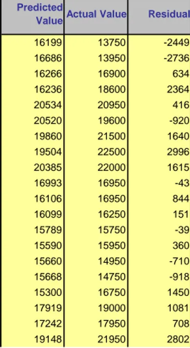
XLMiner produces standard regression output, but we will defer that for now, as well as the more advanced options displayed above. See the chapter on multiple linear regression, or the user documentation for XLMiner, for more information. Rather, we will review the predictions themselves. Here are the predicted values for the first few records in the training data, along with the actual values and the residual (prediction error). Note that these predicted values would often be called the fitted values, since they are for the records that the model was fit to.
2.6 Building a Model ... 27 .
Figure 2.9 And here are the results for the validation data:
Figure 2.10
.
Fgure 2.11
Prediction error can be measured several ways. Three measures produced by XLMiner are shown above.
On the right is the “average error” - simply the average of the residuals (errors). In both cases, it is quite small, indicating that, on balance, predictions average about right - our predictions are “unbiased.” Of course, this simply means that the positive errors and negative errors balance each other out. It tells us nothing about how large those positive and negative errors are.
The “residual sum of squares” on the left adds up the squared errors, so whether an error is positive or negative it contributes just the same. However, this sum does not yield information about the size of the typical error.
The “RMS error” or root mean squared error is perhaps the most useful term of all. It takes the square root of the average squared error, so gives an idea of the typical error (whether positive or negative) in the same scale as the original data.
As we might expect, the RMS error for the validation data ($5,337), which the model is seeing for the first time in making these predictions, is larger than for the training data ($4,518), which were used in training the model.
5. Interpret the results.
At this stage, we would typically try other prediction algorithms (regression trees, for example) and see how they do, error-wise. We might also try different ”settings” on the various models (for example, we could use the ”best subsets” option in multiple linear regression to chose a reduced set of variables that might perform better with the validation data). After choosing the best model (typically, the model with the lowest error while also recognizing that ”simpler is better”), we then use that model to predict the output variable in fresh data. These steps will be covered in more detail in the analysis of cases.
2.7 Exercises 29 6. Deploy the model. After the best model is chosen, it is then applied to new data to predict
MEDV for records where this value is unknown. This, of course, was the overall purpose.
2.6.1
Can Excel Handle the Job?
An important aspect of this process to note is that the heavy duty analysis does not necessarily require huge numbers of records. The data set to be analyzed may have millions of records, of course, but in doing multiple linear regression or applying a classification tree the use of a sample of (say) 20,000 is likely to yield as accurate an answer as using the whole data set. The principle involved is the same as the principal behind polling - 2000 voters, if sampled judiciously, can give an estimate of the entire population’s opinion within one or two percentage points.
Therefore, in most cases, the number of records required in each partition (training, validation and test) can be accommodated within the rows allowed by Excel.
Of course, we need to get those records into Excel, so the standard version of XLMiner provides an interface for random sampling of records from an external database.
Likewise, we need to apply the results of our analysis to a large database, so the standard version of XLMiner has a facility for scoring the output of the model to an external database. For example, XLMiner would write an additional column (variable) to the database consisting of the predicted purchase amount for each record.
2.7
Exercises
1. Assuming that data mining techniques are to be used in the following cases, identify whether the task required is supervised or unsupervised learning:
(a) Deciding whether to issue a loan to an applicant, based on demographic and financial data (with reference to a database of similar data on prior customers).
(b) In an online bookstore, making recommendations to customers concerning additional items to buy, based on the buying patterns in prior transactions.
(c) Identifying a network data packet as dangerous (virus, hacker attack), based on compar-ison to other packets whose threat status is known.
(d) Identifying segments of similar customers.
(e) Predicting whether a company will go bankrupt, based on comparing its financial data to similar bankrupt and non-bankrupt firms.
(f) Estimating the required repair time for an aircraft based on a trouble ticket. (g) Automated sorting of mail by zip code scanning.
(h) Printing of custom discount coupons at the conclusion of a grocery store checkout, based on what you just bought and what others have bought previously.
3. Describe the difference in roles assumed by the validation partition and the test partition. 4. Consider the following sample from a database of credit applicants. Comment on the likelihood
that it was sampled randomly, and whether it is likely to be a useful sample.
Figure 2.12
5. Consider the following sample from a database; it was selected randomly from a larger database to be the training set. “Personal loan” indicates whether a solicitation for a personal loan was accepted and is the response variable. A campaign is planned for a similar solicitation in the future and the bank is looking for a model that will identify likely rsponders. Examine the data carefully and indicate what your next step would be.
2.7 Exercises 31 .
Figure 2.13
6. Using the concept of overfitting, explain why, when a model is fit to training data, zero error with that data is not necessarily good.
7. In fitting a model to classify prospects as purchasers or non-purchasers, a certain company drew the training data from internal data that includes demographic prior and purchase information. Future data to be classified will be purchased lists from other sources with demographic (but not purchase) data included. It was found that “refund issued” was a useful predictor in the training data. Why is this not an appropriate variable to include in the model?
8. A data set has 1000 records and 50 variables. 5% of the values are missing, spread randomly throughout the records and variables. An analyst decides to remove records that have missing values. About how many records would you expect to be removed?
9. Normalize the following data, showing calculations: Age Income 25 $49,000 56 $156,000 65 $99,000 32 $192,000 41 $39,000 49 $57,000
Statistical distance between records can be measured in several ways. Consider Euclidean distance, measured as the square route of the sum of the squared differences. For the first two records above it is:
√[(25−56)2
+ (49,000−156,000)2]
Does normalizing the data change which two records are furthest from each other, in terms of Euclidean distance?
10. Two models are applied to a data set that has been partitioned. Model A is considerably more accurate than model B on the training data, but slightly less accurate than model B on the validation data. Which model are you more likely to consider for final deployment?
11. The data set Auto−NL.xls contains data on used cars (Toyota Corolla) on sale during the late summer of 2004 in the Netherlands. It has 1436 records containing details on 38 attributes includingPrice, Age, Kilometers, Horsepower, and other specifications.
(a) Explore the data using the data visualization (matrix plot) capabilities of the XLMiner. Which of the pairs among the variables seem to be correlated?
(b) We plan to analyze the data using various data mining techniques to be covered in future chapters. Prepare the data for the use as follows:
(i) The data set has two categorical attributes,Fuel−Type(3)andColor(10).
−Describe how you would convert these to binary variables.
−Confirm this using XLMiner’s utility to transform categorical data into dummies.
−How would you work with these new variables to avoid including redundant information in models?
(ii) Prepare the data set (as factored into dummies) for data mining techniques of supervised learning by creating partitions using XLMiner’s data partitioning utility. Select all the variables and use default values for the random seed and partitioning percentages for training (50%), validation (30%) and test (20%) sets. Describe the roles that these partitions will play in modeling.
Chapter 3
Evaluating Classification &
Predictive Performance
In supervised learning, we are interested in predicting the class (classification) or continuous value (prediction) of an outcome variable. In the previous chapter, we worked through a simple example. Let’s now examine the question of how to judge the usefulness of a classifier or predictor and how to compare different ones.
3.1
Judging Classification Performance
Not only do we have a wide choice of different types of classifiers to choose from but within each type of classifier we have many options such as how many nearest neighbors to u