A framework and a web implementation for combinatorial testing

A framework and a web implementation for combinatorial testing

Macario Polo Usaola and Beatriz Pérez Lamancha University of Castilla-La Mancha

Paseo de la Universidad, 4 13071-Ciudad Real (Spain)

Tel.: +34.902.204.100

contact person: [email protected]

Abstract.

Combinatorial strategies have been widely used for test case generation. In spite of this, few available tools exist which put the implementation of such strategies at the disposal of researchers and practitioners. This article provides a short of review of some strategies and makes them available by means of a website with which, further-more, test case source code can be generated by means of a simple (but effective) set of reserved words. All the algorithms are based on a hierarchical class structure that takes advantage of the definitions given in an Algorithm superclass. Moreover, test cases are managed as integer numbers instead of test cases or combinations, which provides additional contributions to the use of time and memory. Additionally, the arti-cle also presents Comb, a new combination strategy which provides quite good results in very little time, as well as a customized version of a pairwise algorithm.

1. INTRODUCTION

According to Myers [1], “a good test case is one that has a high probability of detect-ing an as yet undiscovered error”. Thus, writdetect-ing good test cases requires the execution of the system under test (SUT) in such way that as many errors as possible appear. For this, the SUT’s services must receive, in their parameters, values that try to lead the system into an incorrect or unexpected state, which means that the test case has found an error. In general, a first step for having good test cases is the identification of “good” test values, which are combined in a second step to generate “good” test cases.

• For the first point, techniques such as category-partition, boundary values and error guessing [1] are well known and widely used.

• Once the values have been proposed, they must be adequately combined to obtain good test cases that will probably highlight certain types of errors. Regarding the second point, many errors only arise with the specific interaction of

certain values of two or more parameters, which is one of the fundamentals of combina-torial testing [2]. In this respect, Grindal et al. carried out a literature search and found 16 different combination strategies described in more than 40 papers published between 1985 and 2004, which were reviewed and collected together in a single survey article [3]. Figure 1 reproduces the classification schema of these authors, which categorizes each technique as deterministic or non-deterministic, generally depending on whether the application of the technique always produces the same results with the same input data.

One of the problems with combinatorial testing is finding a compromise between the size of the test suite and its ability to find faults. Take, for example, an object-oriented version of the classic triangle-type determination problem [1]: it consists of a class with three methods to assign values to the three sides of a triangle, plus an additional method to determine its type (an object-oriented version is reported in [4]). Supposing there are four possible values (i.e., {1, 2, 3, 4}) for the three parameters, the most exhaustive test set would be composed of 4×4×4=64 test cases, which proceeds from the application of the Deterministic, Iterative and Test case based technique called “All combinations”. However, many of these test cases will be redundant with respect to others: for exam-ple, the test case with the values {2, 2, 2} (corresponding to an equilateral triangle) will probably not find any error that {1, 1, 1} has not previously found.

On the other hand, the “Each choice” technique, in the same category (Test case based), requires that each test value be included in a test case. This technique produces few test cases: for the triangle problem, {(1, 2, 3), (2, 1, 2), (3, 4, 1), (4, 4, 3)} is a suf-ficient set from the Each choice point of view. However, it is likely that the ability of this test set to find faults in the triangle-type class will be very limited.

Combination strategies

Non-deterministic Deterministic

Heuristic Artificial-_Life based Iterative Instant AETG Simulated Annealing Genetic algorithms Ant colony algorithms Random Test case based Parameter based Orthogonal arrays Covering arrays In parameter order CATS (t-wise) Each choice Partly pair-wise K-bound Antirandom K-perim Base choice All combinations

Figure 1. Classification tree for combination strategies (adapted from [3]). Therefore, each technique may or may not be appropriate for any given software and will have advantages and drawbacks, which are some of most important reasons for researching the development of combination strategies. Indeed, a combination strategy is an algorithm which takes a set of test data as inputs and produces a set of test cases as output: inputs are usually provided by the test engineer, and are the values which pro-ceed from the application of one of the aforementioned basic techniques, or from his/her knowledge and experience. The output is generated according to the rules of the specific combination strategy, and consists of sets of combinations of the values of each input set.

This article describes an object-oriented model for representing combination strate-gies such as those represented in Figure 1, as well as the definition of such algorithms. Some of them have been implemented and released into a reusable Java framework, and published on an operative website which can be freely used by users. Some of the algorithms have been also implemented in Microsoft Excel and can be downloaded from the same site.

One of the core ideas of the article is the possibility of enumerating all the possible combinations by means of an iterative algorithm which implements the All-combinations strategy: since the cardinal of “all All-combinations” is known a priori (the product of the cardinals of all sets), the algorithm makes it possible to obtain an arbi-trary combination given its index. In this way, combinations are actually managed as

integer numbers (instead of sets of values), which has important implications and ad-vantages regarding memory usage and computational costs.

The article also includes two new combination strategies, the first of which is called Comb, whose idea was inspired by the way Antirandom selects test cases [5]. A com-parative analysis of both algorithms is included. The second is a selective pairwise al-gorithm, and proceeds from the actual application of the tool to a software product line project; the idea is to produce pairwise test cases, but exclude any visiting undesired or unneeded pairs.

This article is organized as follows: the next section provides an overview of some techniques used for the validation of testing techniques. Section 3 describes an iterative algorithm to generate all combinations. Section 4 presents the software architecture of the library implemented as well as the implementation of some algorithms. Section 4.7 includes some experimental comparisons of different algorithms. Section 6 lists and explains the three releases of the combinatorial system. Finally, Section 7 describes our conclusions and future lines of work.

2. RELATED WORK

Most likely, the most widely-used technique to assess the quality of test suites and test generation techniques is mutation, a white-box testing technique based on “mu-tants”. A mutant M of a program under test P is a copy of P, but it contains a small change in its code, which is interpreted as a fault. The idea of mutation testing is to write test cases detecting those faults: . simplifying, the more faults found by the test cases, the better the quality of the test suite is. The quality of a test suite is measured in terms of the mutation score, which is the percentage of non-equivalent mutants killed (Figure 2) [6]. ) ( ) , ( E M K T P MS − = _{, where:}

P : program under test T :test suite

K : number of killed mutants M : number of generated mutants E : number of equivalent mutants

Figure 2. Mutation score

On the other hand, when the source code is not available or when, for any reason, the developer of a system is not interested in white-box testing, an additional technique to validate the quality of the testing is the assessment of n-wise coverage. Given a set of parameters, each with a set of values, a test suite covers n-wise if any combination of n

many combination strategies have been proposed which are summarized in an excellent survey published in 2005 [3].

Since this paper deals with combinatorial strategies for test case generation, we focus on the descriptions of the algorithms, on their implementations and on the mechanism used to make them available to the community. The comparisons shown in Section 5 are therefore based on common parameters for this type of strategy, such as generation time and test data pairs visited. The power of each strategy for white-box coverage (for example, detecting the artificial faults injected into mutants) is beyond the scope of this article.

3. ENUMERATION OF ALL COMBINATIONS

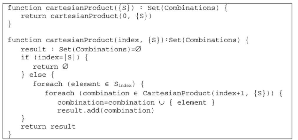
All test cases produced by deterministic strategies are contained in test cases pro-duced by All combinations. Actually, All combinations considers each parameter as a set, and it generates test cases by computing the Cartesian product of all of them. The algorithm for constructing the Cartesian product of n sets is almost trivial: if n is known, only n nested loops are required. Otherwise, it can be easily implemented with recursion: the algorithm in Figure 3 returns the Cartesian product of S, a set of n sets (S={S1, S2, … Sn}). In both cases, the cost of the algorithm is ( | |)

1

∏

function cartesianProduct({S}) : Set(Combinations) { return cartesianProduct(0, {S})

}

function cartesianProduct(index, {S}):Set(Combinations) { result : Set(Combinations)=∅

if (index=|S|) { return ∅ } else {

foreach (element ∈ Sindex) {

foreach (combination ∈ CartesianProduct(index+1, {S})) { combination=combination ∪ { element }

result.add(combination) }

return result }

Figure 3. Recursive algorithm to obtain the Cartesian product of n sets Since the combinations proceeding from the Cartesian product depend on both the number of sets and on the number of elements in each set, it is possible to write a non-recursive algorithm to enumerate all combinations. As an example, Table 2 shows the Cartesian product of the three parameters in Table 1: there are 4*3*2=24 combinations,

each representing a test case.

A={1, 2, 3, 4} B={5, 6, 7} C={8, 9}

Table 1. Three parameters with their test values

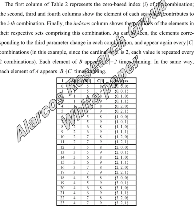
The first column of Table 2 represents the zero-based index (i) of the combination; the second, third and fourth columns show the element of each set which contributes to the i-th combination. Finally, the indexes column shows the positions of the elements in their respective sets comprising this combination. As can be seen, the elements corre-sponding to the third parameter change in each combination, and appear again every |C| combinations (in this example, since the cardinal of C is 2, each value is repeated every 2 combinations). Each element of B appears |C|=2 times running. In the same way, each element of A appears |B|·|C| times running.

i A[i] B[i] C[i] indexes

0 1 5 8 {0, 0, 0} 1 1 5 9 {0, 0, 1} 2 1 6 8 {0, 1, 0} 3 1 6 9 {0, 1, 1} 4 1 7 8 {0, 2, 0} 5 1 7 9 {0, 2, 1} 6 2 5 8 {1, 0, 0} 7 2 5 9 {1, 0, 1} 8 2 6 8 {1, 1, 0} 9 2 6 9 {1, 1, 1} 10 2 7 8 {1, 2, 0} 11 2 7 9 {1, 2, 1} 12 3 5 8 {2, 0, 0} 13 3 5 9 {2, 0, 1} 14 3 6 8 {2, 1, 0} 15 3 6 9 {2, 1, 1} 16 3 7 8 {2, 2, 0} 17 3 7 9 {2, 2, 1} 18 4 5 8 {3, 0, 0} 19 4 5 9 {3, 0, 1} 20 4 6 8 {3, 1, 0} 21 4 6 9 {3, 1, 1} 22 4 7 8 {3, 2, 0} 23 4 7 9 {3, 2, 1}

Table 2. Cartesian product of the sets in Table 1

In general, having n sets {S1, S2, … Sn}, each element of S1 will appear |S2|·|S3|·…·|Sn| times running; elements in S2, |S3|·|S4|…·|Sn|, etc. Elements in Sn appear one time run-ning.

Since the number of combinations is known a priori (

∏

= n i i S 1 |

in-dex i,

∏

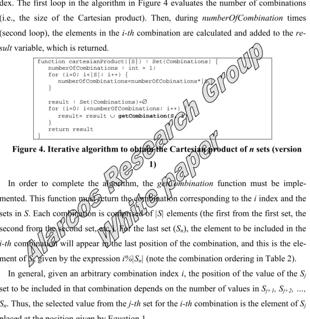
0 , it is possible to know the combination corresponding to that in-dex. The first loop in the algorithm in Figure 4 evaluates the number of combinations (i.e., the size of the Cartesian product). Then, during numberOfCombination times (second loop), the elements in the i-th combination are calculated and added to the re-sult variable, which is returned.

function cartesianProduct({S}) : Set(Combinations) { numberOfCombinations : int = 1;

for (i=0; i<|S|; i++) {

numberOfCombinations=numberOfCobinations*|Si|

}

result : Set(Combinations)=∅

for (i=0; i<numberOfCombinations; i++) { result= result ∪ getCombination(S, i) }

return result }

Figure 4. Iterative algorithm to obtain the Cartesian product of n sets (version 1)

In order to complete the algorithm, the getCombination function must be imple-mented. This function must return the combination corresponding to the i index and the sets in S. Each combination is comprised of |S| elements (the first from the first set, the second from the second set, etc.). For the last set (Sn), the element to be included in the i-th combination will appear in the last position of the combination, and this is the ele-ment of Sn given by the expression i%|Sn| (note the combination ordering in Table 2).

In general, given an arbitrary combination index i, the position of the value of the Sj set to be included in that combination depends on the number of values in Sj+1, Sj+2, …, Sn. Thus, the selected value from the j-th set for the i-th combination is the element of Sj placed at the position given by Equation 1.

| | % ) , ( _j j S divisors i i j TheValue positionOf         = Equation 1

divisorsj is the product of the cardinals from Sj to Sn, and is 1 for Sn. For the example of sets A, B, C (Table 1):

divisorA=|B|·|C|=3·2=6 divisorB=|C|=2 divisorC=1

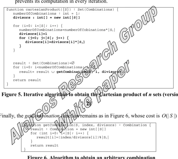
Therefore, the function shown in Figure 4 can be rewritten as in Figure 5: now, the nested loop assigns the corresponding divisor of each set to the divisors variable. Later, in the second outer loop, the getCombination function is called, now with three

parame-ters:

• The set of sets (S)

• The index of the desired combination (i)

• The values of the divisors. Passing this variable as a parameter, the function prevents its computation in every iteration.

function cartesianProduct({S}) : Set(Combinations) { numberOfCombinations : int = 1;

divisors : int[] = new int[|S|]

for (i=0; i<|S|; i++) {

numberOfCombinations=numberOfCobinations*|Si| divisors[i]=1 for (j=0; j<|S|; j++) { divisors[i]=divisors[i]*|Sj] } } result : Set(Combinations)=∅

for (i=0; i<numberOfCombinations; i++) {

result= result ∪ getCombination(S, i, divisors) }

return result }

Figure 5. Iterative algorithm to obtain the Cartesian product of n sets (version 2)

Finally, the getCombination function remains as in Figure 6, whose cost is O(|S|):

function getCombination(S, index, divisors) : Combination { result : Combination = new int[|S|]

for (int i=0; i<|S|; i++) {

result[i]=(index/divisors[i])%|Si|

}

return result }

Figure 6. Algorithm to obtain an arbitrary combination

The cost of the second version of the cartesianProduct algorithm (Figure 5) is also

∏

( , a exponential cost (supposing k elements in every set, is Ο(kn)). How-ever, the cartesianProduct function is iterative and non-recursive, which prevents memory leak problems. Moreover, the getCombination function has an important ad-vantage, which is the possibility of enumerating and recovering any arbitrary combina-tion, given its position. Since the generation of all combinations is not required to re-cover a small set of combinations, this opportunity is quite useful for implementing combination testing strategies, which is the core of this article. On the other hand, since the maximum number of combinations is delimited and known a priori, any combina-tion (or test case) can be uniquely identified by an integer number. This is also an

im-portant contribution from a computational point of view, which is useful for the imple-mentation of other algorithms.

4. IMPLEMENTATION OF STRATEGIES FOR TEST CASE GENERATION

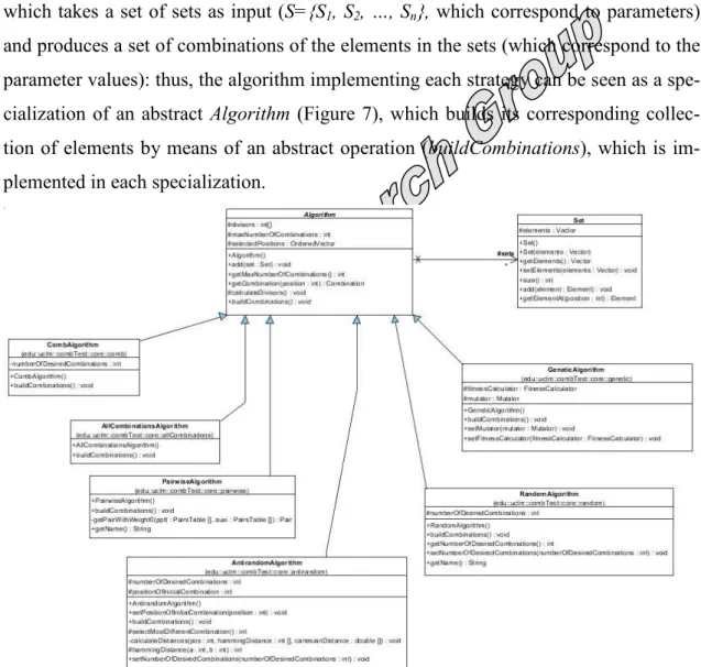
Any of the strategies represented in Figure 1 can be understood as an algorithm which takes a set of sets as input (S={S1, S2, …, Sn}, which correspond to parameters) and produces a set of combinations of the elements in the sets (which correspond to the parameter values): thus, the algorithm implementing each strategy can be seen as a spe-cialization of an abstract Algorithm (Figure 7), which builds its corresponding collec-tion of elements by means of an abstract operation (buildCombinations), which is im-plemented in each specialization.

Figure 7. Hierarchical structure of some algorithms

As seen in the figure, each algorithm holds a collection of sets, which represent the parameters. Moreover, each algorithm has a collection of integers (selectedPositions), which hold the positions of the selected combinations. When recovery of the actual test cases (instances of Combination) is required, each integer in this collection is read and passed as an argument to the function described in Figure 6.

Each Combination keeps an array of as many integers as there are sets in its positions field. Each integer represents the index of the selected element from the corresponding

set. Revisiting Table 2, the first combination holds the values (0, 0, 0) in its positions array and the fifth combination holds the values (0, 2, 1). Given a combination, the al-gorithm extracts the parameter values by visiting its collection of sets.

4.1. Implementation of AllCombinations

With the structure shown in Figure 7, the implementation of any combination strat-egy requires the construction of a subclass of Algorithm. In the case of AllCombina-tions, the required implementation of the inherited buildCombinations operation trans-lates into Java (which is the programming language where the framework is written) the pseudocode shown in Figure 5. In this case, the code of the method is quite simple (Figure 8): note that only integers are added to the selectedPositions set. Later, if the tester is interested in recovering all the combinations, s/he must simply call the get-Combination function (Figure 6) into a loop, passing the index numbers from 0 to num-berOfCombinations-1.

@Override

public void buildCombinations() {

int numberOfCombinations=super.getMaxNumberOfCombinations(); for (int i=0; i<numberOfCombinations; i++) {

this.selectedPositions.add(i);

} }

Figure 8. Implementation of buildCombinations in AllCombinations

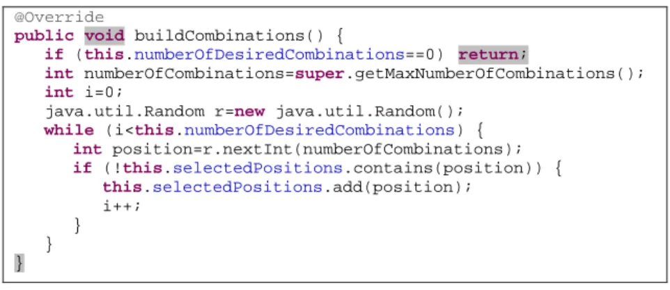
4.2. Implementation of a random algorithm

An algorithm which randomly takes combinations has been also implemented. It takes as input the number of desired combinations, adds random numbers between 0 and numberOfCombinations-1 to selectedPositions and, later, returns the set of test cases corresponding to those positions (Figure 9).

@Override

public void buildCombinations() {

if (this.numberOfDesiredCombinations==0) return;

int numberOfCombinations=super.getMaxNumberOfCombinations(); int i=0;

java.util.Random r=new java.util.Random();

while (i<this.numberOfDesiredCombinations) {

int position=r.nextInt(numberOfCombinations);

if (!this.selectedPositions.contains(position)) {

this.selectedPositions.add(position);

i++; } } }

4.3. Implementation of Antirandom

Antirandom is a test generation technique proposed by Malayia [5]. The algorithm starts with a given test case in the suite (i.e., TS={tc1}); then, the test case most different to tc1 is added to the suite. In a second iteration, the test case most different to the one already selected (let be {tc1, tck}) is added to the suite. The algorithm continues adding, in each iteration, the most different case to the already existing test cases in the suite. The difference between the two test cases is estimated in terms of the Hamming and the Cartesian distances:

1) For the Hamming distance, each test case is codified by a binary vector. The Hamming distance between two binary vectors is the number of bits in which the two vectors differ.

2) The Cartesian distance between two binary vectors is the square root of the Hamming distance.

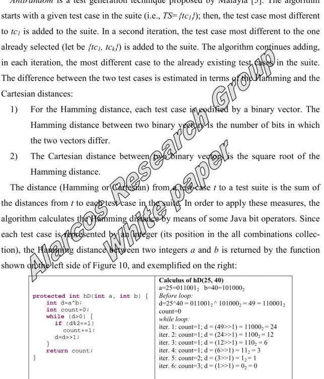
The distance (Hamming or Cartesian) from a test case t to a test suite is the sum of the distances from t to each test case in the suite. In order to apply these measures, the algorithm calculates the Hamming distance by means of some Java bit operators. Since each test case is represented by an integer (its position in the all combinations collec-tion), the Hamming distance between two integers a and b is returned by the function shown on the left side of Figure 10, and exemplified on the right:

protected int hD(int a, int b) { int d=a^b; int count=0; while (d>0) { if (d%2==1) count+=1; d=d>>1; } return count; } Calculus of hD(25, 40) a=25=0110012 b=40=1010002 Before loop: d=25^40 = 0110012 ^ 1010002 = 49 = 1100012 count=0 while loop: iter. 1: count=1; d = (49>>1) = 110002 = 24 iter. 2: count=1; d = (24>>1) = 11002 = 12 iter. 3: count=1; d = (12>>1) = 1102 = 6 iter. 4: count=1; d = (6>>1) = 112 = 3 iter. 5: count=2; d = (3>>1) = 12 = 1 iter. 6: count=3; d = (1>>1) = 02 = 0

Figure 10. Calculus of the Hamming distance between two integers (left) and an example of application (right)

The implementation given to this combination strategy starts by adding either the first combination (#0) or a randomly chosen one to the suite. Then:

1) A loop iterates numberOfDesiredCombinations times and selects the most differ-ent test case, according to the Hamming distance (Figure 11). If there are two combinations with the same Hamming distance, then the selection is made based

on the Cartesian distance (sum of the square roots of the Hamming distance to each preselected test case).

2) When the numberOfDesiredCombinations test cases have been selected, the function stops.

@Override

public void buildCombinations() {

if (this.numberOfDesiredCombinations==0)

return;

int numberOfCombinations=super.getMaxNumberOfCombinations();

int position=this.positionOfInicialCombination==-1 ?

new java.util.Random().nextInt(numberOfCombinations) :

this.positionOfInicialCombination;

this.selectedPositions.add(position);

int i=0;

while (i<this.numberOfDesiredCombinations-1) {

int pos=selectMostDifferentCombination();

if (!this.selectedPositions.contains(pos)) {

this.selectedPositions.add(pos);

i++; } } }

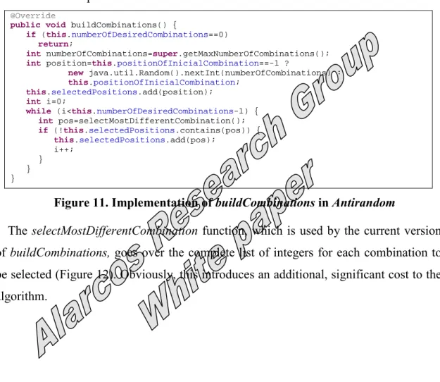
Figure 11. Implementation of buildCombinations in Antirandom

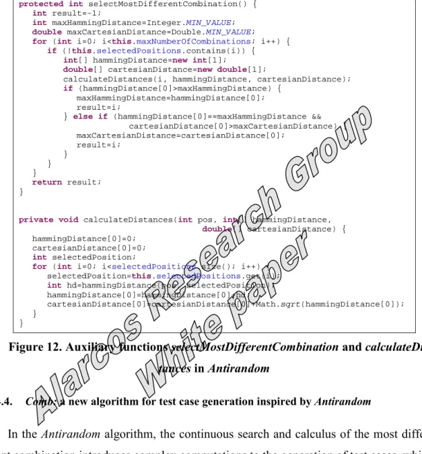
The selectMostDifferentCombination function, which is used by the current version of buildCombinations, goes over the complete list of integers for each combination to be selected (Figure 12). Obviously, this introduces an additional, significant cost to the algorithm.

protected int selectMostDifferentCombination() { int result=-1;

int maxHammingDistance=Integer.MIN_VALUE;

double maxCartesianDistance=Double.MIN_VALUE;

for (int i=0; i<this.maxNumberOfCombinations; i++) {

if (!this.selectedPositions.contains(i)) {

int[] hammingDistance=new int[1];

double[] cartesianDistance=new double[1];

calculateDistances(i, hammingDistance, cartesianDistance); if (hammingDistance[0]>maxHammingDistance) {

maxHammingDistance=hammingDistance[0]; result=i;

} else if (hammingDistance[0]==maxHammingDistance && cartesianDistance[0]>maxCartesianDistance) { maxCartesianDistance=cartesianDistance[0]; result=i; } } } return result; }

private void calculateDistances(int pos, int[] hammingDistance, double[] cartesianDistance) { hammingDistance[0]=0;

cartesianDistance[0]=0; int selectedPosition;

for (int i=0; i<selectedPositions.size(); i++) {

selectedPosition=this.selectedPositions.get(i); int hd=hammingDistance(pos, selectedPosition); hammingDistance[0]=hammingDistance[0]+hd;

cartesianDistance[0]=cartesianDistance[0]+Math.sqrt(hammingDistance[0]); }

}

Figure 12. Auxiliary functions selectMostDifferentCombination and calculateDis-tances in Antirandom

4.4. Comb: a new algorithm for test case generation inspired by Antirandom

In the Antirandom algorithm, the continuous search and calculus of the most differ-ent combination introduces complex computations to the generation of test cases, which makes the progress of this algorithm slow.

However, since we are capable of enumerating all the possible combinations to be generated, the selection of the most different combinations can be made in terms of their index numbers. Thus, in a first iteration, Comb adds the combinations in the first, last and middle positions: supposing there are three sets with 4, 5 and 5 elements, there will be a maximum of 100 combinations: therefore, combinations at positions 0, 99 (the most distant) and 50 (equally distant to the two preselected cases) will be added in a first turn.

Then, in the second iteration, the elements placed in the middle of the intervals [0, 50] and [50, 99] are included. This produces the addition of the combinations 25 and 75.

previous iteration are added to the suite. The algorithm, whose pseudocode appears in Figure 13, stops when a prefixed number of combinations (numberOfDesiredCombina-tions variable) has been reached.

function buildCombinations():Set(Combinations) { result : Set(Combinations)=∅

last : int = getMaxNumberOfCombinations()-1 // zero-based index

result.add(getCombination(0)) // The 1st _{combination is added}

result.add(getCombination(last)) // Also the last combination

p=(last+1)/2

result.add(getCombination(p)) // The middle is also added

while (|result|<numberOfDesiredCombinations) {

k : float = p/2 // k moves by the middle point

of each interval counter : int = 2

while (k<last && |result|<numberOfDesiredCombinations) { c : Combination = getCombination(k)

if (c∉result) result.add(c)

k = counter *(p/2) // when k is multiplied by counter,

it advances to the next interval counter = counter +1 } p = p /2 } return result }

Figure 13. Pseudocode of buildCombinations for the Comb algorithm Assuming the aforementioned 100 combinations, the application of the algorithm is illustrated in Figure 14. Before entering the first while loop, combinations 0, 50 and 99 are added, in the first iteration, 25 and 75 and in the second one, 12, 37, 62 and 87. The variables change according to Table 3. The evolution of the selected positions along the line in Figure 14 may remind one of the teeth on a comb, which is the reason that this name was given to the algorithm.

p k counter

index of c

(selected combination) result

50.0 25.0 2 25 {0, 99, 50} 50.0 3 50 {0, 99, 50, 25} 75.0 4 75 {0, 99, 50, 25, 75} 25.0 12.5 2 12 {0, 99, 50, 25, 75, 12} 25.0 3 25 {0, 99, 50, 25, 75, 12} 37.5 4 37 {0, 99, 50, 25, 75, 12, 37} 50.0 5 50 {0, 99, 50, 25, 75, 12, 37} 62.5 6 62 {0, 99, 50, 25, 75, 12, 37, 62} 75.0 7 75 {0, 99, 50, 25, 75, 12, 37, 62} 87.5 8 87 {0, 99, 50, 25, 75, 12, 37, 62, 87} 12.5 6.25 2 6 {0, 99, 50, 25, 75, 12, 37, 62, 87, 6} 12.5 3 12 {0, 99, 50, 25, 75, 12, 37, 62, 87, 6} 18.75 4 18 {0, 99, 50, 25, 75, 12, 37, 62, 87, 6, 18} 25.0 5 25 {0, 99, 50, 25, 75, 12, 37, 62, 87, 6, 18} 31.25 6 31 {0, 99, 50, 25, 75, 12, 37, 62, 87, 6, 18, 31} 37.5 7 37 {0, 99, 50, 25, 75, 12, 37, 62, 87, 6, 18, 31} 43.75 8 43 {0, 99, 50, 25, 75, 12, 37, 62, 87, 6, 18, 31, 43} … … … … …

Table 3. Evolution of the variables with the Comb algorithm

Figure 14. Illustration of the Comb algorithm

4.5. Implementation of a basic Pairwise algorithm

Pairwise algorithms generate test cases with the goal of visiting all the pairs of the parameter values. For this, a basic implementation of a pairwise algorithm builds all the pair tables (n·(n-1)/2, being n the number of sets) for all the sets. Each pair contains the positions of the two elements of the two sets. For the example of the three sets in Table 1, the three pair tables shown in Table 4 are created.

A,B (1, 5) (1, 6) A,C (1, 7) (1, 8) B,C (2, 5) (1, 9) (5, 8) (2, 6) (2, 8) (5, 9) (2, 7) (2, 9) (6, 8) (3, 5) (3, 8) (6, 9) (3, 6) (3, 9) (7, 8) (3, 7) (4, 8) (7, 9) (4, 5) (4, 9) (4, 6) (4, 7)

Table 4. Pair tables for the A, B, C sets of Table 1

While there are non-used pairs in the tables, the algorithm (Figure 15) looks for the pairs with fewest visits and uses them to construct the new test case.

function buildCombinations():Set(Combinations) { result : Set(Combinations)=∅

pairsTables : Set(PairTable) = buildPairsTables() Pair p;

while (p=pairsTables.getPairWithWeight(0)!=null) { min : int = ∝

for (i=0; i<maxNumberOfCombinations; i++) { c : Combination = getCombination(i)

weightOfPairs : int = c.getWeight(pairsTables) if (c.contains(p) && weightOfPairs<min) {

selectedCombination = c min=weightOfPairs } } selectedCombination.visitPairs(pairsTables) result.add(selectedCombination) } return result }

Figure 15. Pseudocode of buildCombinations for the Pairwise algorithm For the example in Table 4, the algorithm takes the first non-visited pair ((1,5)) in the (A,B) table and looks for a compatible non-visited pair in (A,C) and (B,C). The (1,5) pair in (A,B) respectively involves elements 1 and 5 from A and B. Therefore, a pair (1,X) and (5, Y) must be taken from (A, C) and (B, C), for example, (1,8) and (5,8). This produces the test case formed by the test values (1, 5, 8).

Additionally, the implementation given to the PairwiseAlgorithm (an specialization of the abstract Algorithm shown in Figure 7) saves, in addition to the generated test cases, the number of uses of each pair (Table 5).

Test cases A,B 0-> {1, 5, 8} (1, 5), 1 1-> {1, 6, 9} (1, 6), 1 A,C 2-> {1, 7, 8} (1, 7), 1 (1, 8), 2 B,C 3-> {2, 5, 9} (2, 5), 1 (1, 9), 1 (5, 8), 2 4-> {2, 6, 8} (2, 6), 1 (2, 8), 1 (5, 9), 2 5-> {2, 7, 9} (2, 7), 1 (2, 9), 2 (6, 8), 2 6-> {3, 5, 8} (3, 5), 1 (3, 8), 2 (6, 9), 2 7-> {3, 6, 9} (3, 6), 1 (3, 9), 1 (7, 8), 2 8-> {3, 7, 8} (3, 7), 1 (4, 8), 1 (7, 9), 2 9-> {4, 5, 9} (4, 5), 1 (4, 9), 2 10-> {4, 6, 8} (4, 6), 1 11-> {4, 7, 9} (4, 7), 1

Table 5. Test cases generated (table in the left) and number of uses of each pair

4.6. Implementation of AETG

AETG is an algorithm proposed by Cohen et al. [7] for covering n-wise. The imple-mentation we have given this algorithm produces pairwise coverage. Cohen et al. de-scribe the algorithm as in Figure 16.

Assume that we have a system with k test parameters and that the i-th parameter has li different values. Assume that we have already selected r test cases. We select the r + 1 by first generating M different candidate test cases and then choosing one that covers the most new pairs. Each candidate test case is selected by the following greedy algo-rithm:

1.Choose a parameter f and a value l for f such that that parameter value appears in the greatest number of uncovered pairs.

2.Let f1 = f. Then choose a random order for the remaining parameters. Then, we have an order for all k parameters f1, ..., fk.

3.Assume that values have been selected for parameters f1, ..., fj. For 1 ≤ i ≤ j, let the selected value for fi be called vi. Then, choose a value vj+1 for fj+1 as fol-lows. For each possible value v for fj, find the number of new pairs in the set of pairs {fj+1 = v and fi = vi for 1 ≤ i ≤ j}. Then, let vj+1 be one of the values that appeared in the greatest number of new pairs.

Note that, in this step, each parameter value is considered only once for inclu-sion in a candidate test case. Also, that when choosing a value for parameter fj+1, the possible values are compared with only the j values already chosen for parameters f1,..., fj.

Figure 16. Original explanation of the AETG algorithm for covering pairwise [7] Note there is a random ordering of the parameters in the second step. In order to al-low the reproducibility of test generation, we have removed that chance with no loss of validity in our implementation (Figure 17).

1. Build pairTables for S, the set of sets/parameters 2. let c=combination #0

3. Add c to the selected set

4. Update pairTables with the pairs visited by c 5. while there are unvisited pairs in pairTables

1. initialize c putting the value which visits more unvisited pairs in pairTables

2. complete c with the values of the remaining sets in such way most pairs are jointly visited

3. Add c to the selected set

4. Update pairTables with the pairs visited by c Figure 17. Pseudocode of the implementation given to AETG

Thus, assuming the three sets of Table 1 (A={1, 2, 3}, B={4, 5}, C={6, 7}), the algo-rithm initially builds the pair tables. Then, the first combination (#0, since it is zero-based) is added to the selected set, which corresponds to elements {1, 4, 6}. The pair tables are updated with the visits made by combination #0, and the visited pairs are marked (Figure 18): 6 pairs in (A, B) Elements # of visits (1, 4) 1 (1, 5) 0 (2, 4) 0 (2, 5) 0 (3, 4) 0 (3, 5) 0 6 pairs in (A, C) Elements # of visits (1, 6) 1 (1, 7) 0 (2, 6) 0 (2, 7) 0 (3, 6) 0 (3, 7) 0 4 pairs in (B, C) Elements # of visits (4, 6) 1 (4, 7) 0 (5, 6) 0 (5, 7) 0

Figure 18. Pairs visited by the first combination Then:

1. A new combination is initialized. The selected element is that of the three sets which visits the most unvisited pairs. In this case, the selected element is the second element of the B set (#1, since it is zero-based). Thus, the candidate combination is c={-, 5, -}

2. To know the most suitable value of the first set (A) to be included as the first element of c, the algorithm considers all the elements of A, and checks how ma-ny unvisited pairs each element of A visits with the selected element of B. That

is, it counts the pairs visited in (1, 5), (2, 5) and (3, 5) (in the table correspond-ing to parameters (A, B)). The algorithm selects the first element of A (1). 3. To know the most suitable value of the third set to be included as the third

ele-ment of c, the algorithm considers all the eleele-ments of C, and checks how many unvisited pairs each element of C visits with the selected elements of A and B. That is, in table (A, C) it counts the pairs visited by 1 in the pairs (1, 6) and (1, 7) (it uses 1 in A because it has been previously selected).

In table (B, C), it considers the pairs (5, 6) and (5,7).

In this example, the algorithm selects the second element of C (7).

4. The combination is now completed, and it is comprised of the values (1, 5, 7). It is added to the selected set and the pair tables are updated with the pairs vis-ited by this combination (Figure 19).

6 pairs in (A, B) Elements # of visits (1, 4) 1 (1, 5) 1 (2, 4) 0 (2, 5) 0 (3, 4) 0 (3, 5) 0 6 pairs in (A, C) Elements # of visits (1, 6) 1 (1, 7) 1 (2, 6) 0 (2, 7) 0 (3, 6) 0 (3, 7) 0 4 pairs in (1, 2) Elements # of visits (4, 6) 1 (4, 7) 0 (5, 6) 0 (5, 7) 1

Figure 19. Pairs visited by the second selected combination

5. Later, the algorithm again looks for the element (in any set) which visits more unvisited pairs, selecting element 3 from the A set: c={3, -, -}.

6. The second and third positions of c must be completed. For this, the algorithm looks at what elements in B, together with the selected element of A (3, in this case) visit more pairs. From B, the algorithm selects element 4.

In the same way, it looks for the element in C which visits more pairs, taking into account that the selected element of A is 3 and that the selected element of B is 4. Therefore, it selects number 7 from C and leaves c with the values (3, 4, 7).

7. The algorithm continues in this way until all pairs have been visited. The final results are: {1, 4, 6}, {1, 5, 7}, {3, 4, 7}, {3, 5, 6}, {2, 4, 6} and {2, 5, 7}.

4.7. Implementation of a customized pairwise

One of the research lines we are currently developing is the automatic generation of test cases in Software Product Lines (SPL). Products in an SPL share a set of character-istics (commonalities) and differ in a number of variation points, which represent the variabilities of the products. Commonalities represent assumptions that are true for each member of the SPL, whilst variabilities are a structured list of assumptions on how the family members (products) differ [8]. Software construction in SPL contexts involves two levels: (1) Domain Engineering, referring to the development of common features and the identification of variation points and (2) Product Engineering, where each spe-cific product is built, which leads to the inclusion of the commonalities in the products, and the corresponding adaptation of the variation points.

Our SPL makes it possible to play a set of board games (Ludo, Trivial Pursuit, Chess and Checkers). All these games share a set of characteristics (identification of the play-ers, turn management, etc.). Ludo and Trivial require dice, but not Chess nor Checkers. Trivial Pursuit also requires a quiz with the corresponding questions. Chess and Check-ers require two playCheck-ers, but the othCheck-ers may accept more. Thus, initially we have sets with games, dice, a quiz and a number of players. It is interesting to test the possible pair combinations, but some of them will not belong to some final products (for exam-ple, Chess with Dice and 3 players). Therefore, with our customized pairwise algorithm those pairs which will not be interesting can be excluded.

Firstly, the algorithm asks the user to mark the unneeded pairs. Then, it builds all the combinations with the iterative All combinations algorithm. Finally, it removes those combinations which hold undesired pairs.

4.8. Implementation of Each choice

This is a very basic algorithm proposed by Amman and Offutt [9]. According to [3], the basic idea behind the Each Choice combination strategy is to include each value of each parameter in at least one test case. This is achieved by generating test cases by successively selecting unused values for each parameter.

Thus, the algorithm is very simple: while there are unvisited values, a new combina-tion is built. If a set has any unused value, it is inserted in the combinacombina-tion; otherwise, a random value is picked up.

5. EXPERIMENTAL RESULTS

This section shows the results of some experiments comparing two pairs of rithms of the same nature. On the one hand, the basic pairwise and the AETG algo-rithms and on the other, the Antirandom and Comb algoalgo-rithms.

All computations have been locally executed on a standard PC with a Pentium Core Duo processor, a speed of 2.4 Ghz and 4 Mb of RAM memory.

5.1. Cost and result comparison of the basic pairwise algorithm and AETG

Both the basic pairwise (Section 4.5) and AETG (Section 4.6) algorithms obtain pairwise coverage, i.e., they visit all the pairs of parameter values in the pair tables. The problem with generating a test suite with the minimal possible size which visits all the pairs is NP-complete, and there have been several proposals for algorithms to find near-to-the-optimal solutions.

Thus, the comparison of pairwise algorithms can be done based on three variables: 1) Execution time.

2) Test suite size.

3) Total number of visits to pairs.

In a first experiment, we have built pairwise test cases using from 3 to 5 sets. All the sets have the same number of parameters, from 5 to 20. The results of the time com-parison in milliseconds appear in Figure 20 and Figure 21. Note the exponential growth of the basic pairwise strategy.

0 200000 400000 600000 800000 1000000 1200000 1400000 1600000 1800000

5 6 _{PW time (3 sets)}7 8 9 10 11 12_{AETG time (3 sets)}13 14 15 16 17 18 19 20

PW time (4 sets) AETG time (4 sets)

Figure 20. Time comparison between basic pairwise and AETG for 3 and 4 equ-ally-sized sets 0 2000000 4000000 6000000 8000000 10000000 12000000 5 6 7 8 9 10 11 12 13 14 15 16 17

PW time (5 sets) AETG time (5 sets)

Figure 21. Time comparison between basic pairwise and AETG for 5 equally-sized sets

Regarding the test suite size and the total number of visits, basic pairwise exhibits slightly better results than AETG which, however, do not compensate for the execution time (Table 6).

Pair visits |Test suite| Sets # of elements PW AETG PW AETG

3 5 84 84 28 28 3 6 120 123 40 41 3 7 159 159 53 53 3 8 192 192 64 64 3 9 264 264 88 88 3 10 336 339 112 113 3 11 411 417 137 139 3 12 480 492 160 164 3 13 567 567 189 189 3 14 636 648 212 216 3 15 708 708 236 236 3 16 768 768 256 256 3 17 912 912 304 304 3 18 1056 1059 352 353 3 19 1203 1209 401 403 3 20 1344 1356 448 452 4 5 180 186 30 31 4 6 276 270 46 45 4 7 384 360 64 60 4 8 576 474 96 79 4 9 612 588 102 98 4 10 732 756 122 126 4 11 852 888 142 148 4 12 864 1056 144 176 4 13 1164 1254 194 209 4 14 1344 1404 224 234 4 15 1524 1590 254 265 4 16 1536 1794 256 299 4 17 1950 2064 325 344 4 18 2244 2322 374 387 4 19 2532 2610 422 435 4 20 2928 2880 488 480 5 5 330 340 33 34 5 6 480 520 48 52 5 7 670 690 67 69 5 8 960 860 96 86 5 9 1060 1090 106 109 5 10 1300 1370 130 137 5 11 1520 1630 152 163 5 12 2400 1900 240 190 5 13 2070 2190 207 219 5 14 2380 2540 238 254 5 15 2730 2940 273 294 5 16 2560 3260 256 326 5 17 3380 3740 338 374

Table 6. Comparison of visits and test suite size (basic pairwise and AETG) for equally-sized sets

num-ber of elements (between 3 and 10). The results, shown in Table 7, are quite similar to the previous ones.

Time (milliseconds) Visits |Test suite|

Sets # of elements PW AETG PW AETG PW AETG

3 5,9,4 91.47 35.43 135 135 45 45 3 9,3,4 49.72 19.30 108 108 36 36 3 7,9,7 368.64 92.84 201 201 67 67 4 10,3,5,10 2,304.89 222.08 600 600 100 100 4 11,3,7,4 931.02 120.65 462 462 77 77 4 8,4,7,11 3,877.22 231.98 558 534 93 89 5 8,9,3,11,11 110,521.25 712.48 1290 1280 129 128 5 5,8,9,5,9 38,016.90 296.98 940 900 94 90 5 6,7,11,10,7 119,861.91 549.15 1180 1120 118 112 6 10,8,11,7,10,9 785,156.08 1,525.25 1905 1965 127 131 6 6,10,10,9,4,6 113,322.18 689.79 1650 1560 110 104 6 10,9,11,9,4,7 277,374.96 1,043.58 1860 1755 124 117 7 8,8,9,9,9,10,7 315,476.87 1,740.98 2436 2499 116 119 7 5,9,4,5,10,8,6 396,215.42 698.74 2142 2016 102 96 7 5,6,9,7,6,4,3 71,730.80 326.10 1554 1386 74 66

Table 7. Time results in the second experiment

5.2. Cost and result comparison of Antirandom and Comb

Since the nature of Antirandom and Comb looks similar (selection of test cases as far from the previously selected ones as possible), it is interesting to compare their per-formance and the quality of the test cases produced. In order to do this comparison, we applied both algorithms to generate several test suites from different sets with different numbers of parameters.

In the first experiment, we used from 2 to 7 sets (parameters) with 5 to 10 elements (test values). Then, the two algorithms were executed. We collected the execution time (in seconds) of each algorithm and the percentage of pairs visited in the selected test suite. In this experiment, we generated test suites with 2|Sets| test cases, since this is the number of test cases used in the original work by Malayia [5]. The results are shown in Table 8:

1) With respect to time, note the exponential growth of Antirandom.

2) With respect to pairs, Figure 22 shows how, when the number of sets and their sizes are small, the pairwise coverage is almost equal. As these factors increase, Comb provides, in general, better results.

Antirandom Comb Sets Sets

size Combinations Time

% pairs visited Time % pairs visited 2 5 4 0.002489 16.04 0.000138 16.00 2 6 4 0.002729 11.11 0.000148 11.11 2 7 4 0.001842 8.16 0.000064 8.16 2 8 4 0.002099 6.25 0.000061 6.25 2 9 4 0.002399 4.94 0.00005 4.94 2 10 4 0.001755 4.04 0.000046 4.00 3 5 8 0.008911 30.67 0.000184 29.33 3 6 8 0.010766 20.37 0.000158 19.44 3 7 8 0.006817 15.65 0.000142 15.65 3 8 8 0.010772 9.38 0.000166 9.38 3 9 8 0.01511 9.05 0.000189 9.88 3 10 8 0.01916 7.67 0.000154 7.00 4 5 16 0.04697 46.67 0.00043 58.67 4 6 16 0.086497 32.87 0.000436 31.02 4 7 16 0.165528 25.17 0.00044 26.53 4 8 16 0.252096 11.98 0.000448 10.94 4 9 16 0.41097 17.08 0.000433 16.87 4 10 16 0.63463 15.83 0.000389 11.83 5 5 32 0.634861 52.43 0.001204 86.80 5 6 32 1.600526 49.44 0.001232 45.56 5 7 32 3.676166 26.12 0.000987 54.08 5 8 32 4.712947 15.31 0.001011 12.50 5 9 32 8.938747 24.69 0.000522 34.44 5 10 32 15.874164 19.23 0.000546 19.10 6 5 64 11.11741 74.46 0.002926 94.67 6 6 64 23.810523 71.48 0.002224 57.59 6 7 64 63.219331 49.12 0.001898 85.58 6 8 64 145.278813 25.42 0.001962 15.42 6 9 64 330.109692 27.00 0.001585 64.53 6 10 64 622.283298 33.26 0.001631 29.87 7 5 128 152.249373 67.62 0.007992 95.24 7 6 128 601.914038 58.60 0.008475 65.21 7 7 128 1925.366244 51.21 0.00872 99.13 7 8 128 5111.97125 31.85 0.010736 14.43 7 9 128 12961.39864 43.33 0.008688 93.71

0.00 20.00 40.00 60.00 80.00 100.00 120.00 1 3 5 7 9 11 13 15 17 19 21 23 25 27 29 31 33 35 AR pairs Comb pairs

Figure 22. Pairwise coverage of Antirandom and Comb in the first experiment In the second experiment, instead of generating 2|Sets| test cases, we generated from 10 to 95 test cases in 5 and 6 sets with 5 elements each. As seen in Figure 23, the dif-ference in time (in seconds) is also significant. Regarding pairwise coverage, Figure 24 clearly shows how Comb always obtains better results than Antirandom, quickly evolv-ing to 100%, which seems to be its asymptote.

0 2000 4000 6000 8000 10000 12000 14000 16000 18000 1 2 3 4 5 6 7 8 9 10 11 12 13 14 15 16 17 18 AR time (5 sets) Comb time (5 sets) AR time (6 sets) Comb time (6 sets)

0 20 40 60 80 100 120 1 2 3 4 5 6 7 8 9 10 11 12 13 14 15 16 17 18 AR pairs (5 sets) Comb pairs (5 sets) AR pairs (6 sets) Comb pairs (6 sets)

Figure 24. Pairs visited in the second experiment

6. IMPLEMENTATIONS

To allow both the research and the practitioner communities the use of these algo-rithms, we released them on a website (http://alarcosj.esi.uclm.es/CTWeb).

1) First, the algorithms are packaged as a Java library to allow their reuse in other applications, as well as the proposal of new combination strategies by means of the implementation of new subclasses of Algorithm.

2) Second, some of the algorithms are available in Microsoft Excel files. In this way, any user may fill in some cells in a spreadsheet and select the desired combination strategy to obtain the desired combinations.

3) Third, the URL includes a web application where the user can create any num-ber of parameters, adding values and applying any combination strategy (Figure 25). The web application includes a “verbose” option, which explains how each algorithm produces the results. Note that the web application includes the pos-sibility of generating code for the test cases corresponding to each selected combination: the text area under the sets allows the tester to introduce a tem-plate text. The tester uses the TCNUMBER reserved word to reference the test case number, and #A, #B, #C, etc. to reference the corresponding value of each set in the selected combination. When test cases have been generated, the appli-cation substitutes these tokens with the corresponding test values and shows the

corresponding code on the webpage. Then, this code can be easily copied and pasted into the development environment to perform the tests.

Figure 25. An excerpt of the web application

7. CONCLUSIONS

This article has shown and made available the implementations of several algorithms for test case generation. The article also provides details of the class structure of the application architecture. To the best of our knowledge, this is the first work to provide so many open implementations of so many combination strategies. Our goal is to give researchers and practitioners a system for (1) developing new testing strategies within a framework, which easily allows for comparison and (2) testing actual programs.

In another respect, the use of the web application is also highly recommended for teaching in testing courses, both at graduate and postgraduate levels. In fact, we are currently using it in a PhD course at the University of Castilla-La Mancha, with the students expressing a high degree of satisfaction. The “verbose” option of the

applica-tion is useful for understanding how algorithms work.

One of the principles of all algorithms is the method for obtaining an arbitrary com-bination (i.e., an arbitrary element of the Cartesian product) by means of its simple enumeration. In the case of the All combinations algorithm, and even though its cost is exponential, the iterative nature of the given implementation and the possibility of re-covering any combination from its index helps with the computational behaviour and prevents problems of memory leaks. Moreover, the fact of dealing with simple integer numbers instead of test cases or combination objects also improves the performance of all of the algorithms.

Additional contributions of the paper are the Comb and the customizable pairwise al-gorithms. The former proceeds from an idea similar to that of Antirandom, although it produces better results in much less time. The latter comes from the actual application of combination testing to the development of a software product line. One of our future works is the comparison of Comb with other algorithms using a white-box criterion, such as the mutation score. Regarding the web application, we are already working on the addition of a module to upload a .class file; by reusing the bytecode analysis tech-niques implemented in testooj [10], the tool will show the list of operations in the class. Then, the tester will be able to write a regular expression to generate tests, as well as add test values to parameters.

It is our desire that both researchers and practitioners make use of the combinatorial testing web site.

8. ACKNOWLEDGMENTS

This work is partially supported by the PRALÍN (Junta de Comunidades de Castilla-La Mancha/European Social Fund, grant PAC08-121-1374), DIMITRI (MI-CINN/FEDER, TRA2009_0131) and PEGASO/MAGO (MI(MI-CINN/FEDER, TIN2009-13718-C02-01) projects.

The authors would like to thank José Antonio Cruz for his help in the implementa-tion of the Excel versions of the algorithms.

9. REFERENCES

1. Myers B (2004). The Art of Software Testing, second edition. Hoboken, New Jersey: Wiley. 2. Bryce RC, Lei Y, Kuhn DR and Kacker R (2010). Combinatorial testing. En Software Engi-neering and Productivity Technologies, M. Ramachandran and R.A.d. Carvalho (eds.). Idea Group Pub-lishing. p. 196-208.

Verification and Reliability, 15(167-199, 2005.

4. Polo M, Piattini M and García-Rodríguez I. Decreasing the cost of mutation testing with second-order mutants. Software Testing, Verification and Reliability, 19(2), 111-131, 2008.

5. Malaiya Y. Antirandom testing: Getting the most out of black-box testing. International Sym-posium on Software Reliability Engineering (ISSRE 95). Toulouse, France, pp. 86-95. IEEE Computer Society Press, Los Alamitos, CA, 1995.

6. Hamlet R. Testing programs with the help of a compiler. IEEE Transactions on Software Engi-neering, 3(4), 279-290, 1977.

7. Cohen DM, Dalal SR, Parelius J and Patton GC. The combinatorial design approach to auto-matic test generation. IEEE Transactions on Software Engineering, 13(5), 83-89, 1996.

8. Trigaux J and Heymans P. Modelling variability requirements in Software Product Lines: A comparative survey. FUNDP–Equipe LIEL, Namur, 2003.

9. Ammann P and Offutt AJ. Using formal methods to derive test frames in category-partition testing. Ninth Annual Conference on Computer Assurance (COMPASS'94). Gaithersburg, MD, pp. 69-80. IEEE Computer Society Press, Los Alamitos, CA, 1994.

10. Polo M, Piattini M and Tendero S. Integrating techniques and tools for testing automation. Soft-ware Testing, Verification and Reliability, 17(1), 3-39, 2007.