Integration of Massive Plug-in Hybrid Electric Vehicles into Power Distribution Systems: Modeling, Optimization, and Impact Analysis

(1)

University of Wisconsin Milwaukee

UWM Digital Commons

Theses and Dissertations

May 2017

Integration of Massive Plug-in Hybrid Electric

Vehicles into Power Distribution Systems:

Modeling, Optimization, and Impact Analysis

Jun Tan

University of Wisconsin-Milwaukee

Follow this and additional works at:https://dc.uwm.edu/etd

Part of theElectrical and Electronics Commons

This Dissertation is brought to you for free and open access by UWM Digital Commons. It has been accepted for inclusion in Theses and Dissertations by an authorized administrator of UWM Digital Commons. For more information, please [email protected].

Recommended Citation

Tan, Jun, "Integration of Massive Plug-in Hybrid Electric Vehicles into Power Distribution Systems: Modeling, Optimization, and Impact Analysis" (2017).Theses and Dissertations. 1545.

(2)

INTEGRATION OF MASSIVE PLUG-IN HYBRID ELECTRIC VEHICLES

INTO POWER DISTRIBUTION SYSTEMS: MODELING, OPTIMIZATION,

AND IMPACT ANALYSIS

by

Jun Tan

A Dissertation Submitted in

Partial Fulfillment of the

Requirements for the Degree of

Doctor of Philosophy

in Engineering

at

The University of Wisconsin-Milwaukee

(3)

ABSTRACT

INTEGRATION OF MASSIVE PLUG-IN HYBRID ELECTRIC VEHICLES INTO POWER DISTRIBUTION SYSTEMS: MODELING, OPTIMIZATION, AND IMPACT ANALYSIS

by Jun Tan

The University of Wisconsin-Milwaukee, 2017 Under the Supervision of Professor Lingfeng Wang

With the development of vehicle-to-grid (V2G) technology, it is highly promising to use plug-in hybrid electric vehicles (PHEVs) as a new form of distributed energy resources. However, the uncertainties in the power market and the conflicts among different stakeholders make the integration of PHEVs a highly challenging task. Moreover, the integration of PHEVs may lead to negative effects on the power grid performance if the PHEV fleets are not properly managed.

This dissertation studies various aspects of the integration of PHEVs into power distribution systems, including the PHEV load demand modeling, smart charging algorithms, frequency regulation, reliability-differentiated service, charging navigation, and adequacy assessment of power distribution systems. This dissertation presents a comprehensive methodology for modeling the load demand of PHEVs. Based on this stochastic model of PHEV, a two-layer evolution strategy particle swarm optimization (ESPSO) algorithm is proposed to integrate PHEVs into a residential distribution grid. This dissertation also develops an innovative load frequency control system, and proposes a hierarchical game framework for PHEVs to optimize

(4)

their charging process and participate in frequency regulation simultaneously. The potential of using PHEVs to enable reliability-differentiated service in residential distribution grids has been investigated in this dissertation. Further, an integrated electric vehicle (EV) charging navigation framework has been proposed in this dissertation which takes into consideration the impacts from both the power system and transportation system. Finally, this dissertation proposes a comprehensive framework for adequacy evaluation of power distribution networks with PHEVs penetration.

This dissertation provides innovative, viable business models for enabling the integration of massive PHEVs into the power grid. It helps evolve the current power grid into a more reliable and efficient system.

(5)

(6)

To my parents, my parents in law,

my wife

(7)

LIST OF FIGURES

Figure 2. 1 Percentage of vehicles versus their departure time ... 10

Figure 2. 2 Percentage of vehicles versus their arrival time. ... 10

Figure 2. 3 Percentage of vehicles versus daily miles driven. ... 10

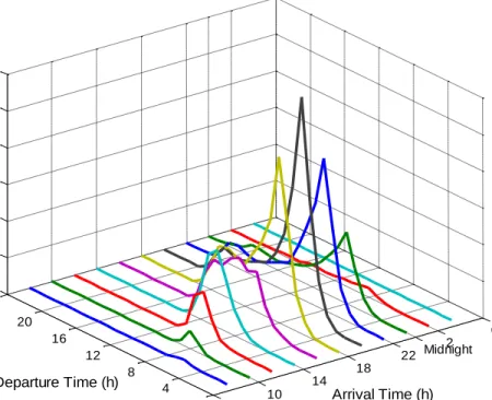
Figure 2. 4 PDF of departure time at different time windows of arrival time. ... 11

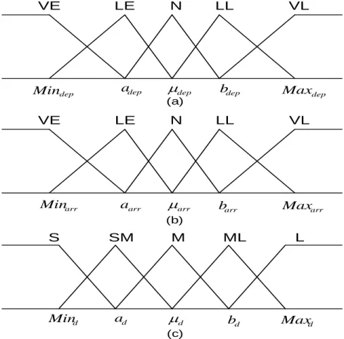
Figure 2. 5 Fuzzy membership functions. (a) Departure time pattern. (b) Arrival time pattern. (c) Daily travel mileage pattern. ... 13

Figure 2. 6 Convergence curve of the PSO algorithm. ... 15

Figure 2. 7 The PHEV load profile modeling framework. ... 18

Figure 3. 1 The principle of dominant solution matrix………..24

Figure 3. 2 The topology of the studied residential distribution grid. ... 27

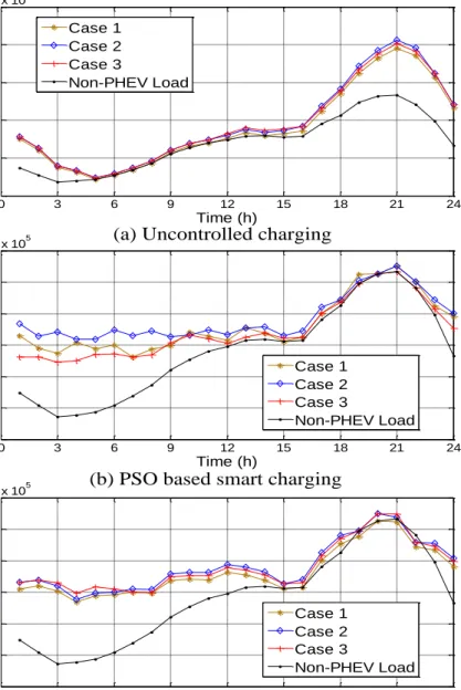
Figure 3. 3 Load demand curves of the tested system with different PHEV modeling methods and control strategies. ... 28

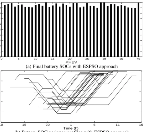
Figure 3. 4 Final battery SOCs and battery SOC variance profiles with ESPSO approach at 10% PHEV penetration level. ... 30

Figure 3. 5 Virtual time-of-use rate for different control strategies at 20% PHEV penetration level. ... 30

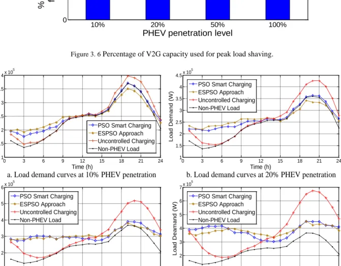
Figure 3. 6 Percentage of V2G capacity used for peak load shaving. ... 31

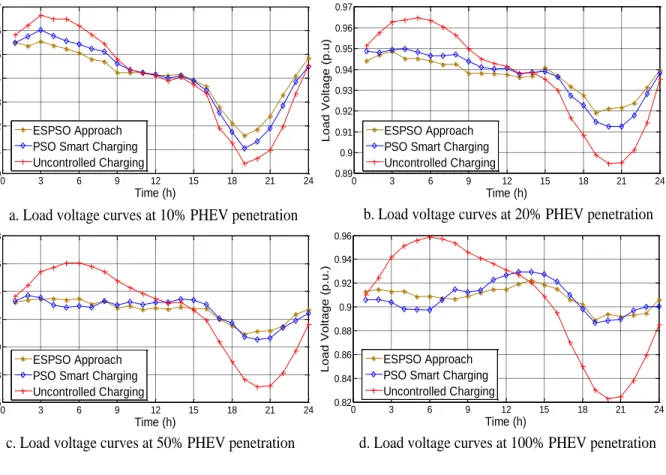
Figure 3. 7 Load demand curves of the studied system for different charging algorithms at different PHEV penetration levels. ... 31

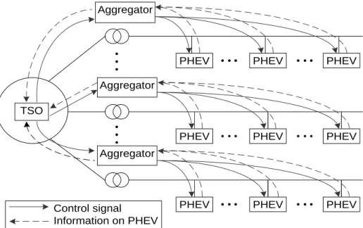
Figure 3. 8 Voltage curves of node 34 for different charging algorithms at different PHEV penetration levels. ... 32

(13)

Figure 4. 1 LFC model with PHEV aggregators………36

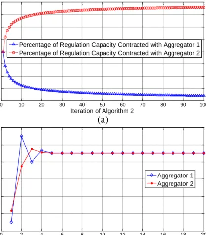
Figure 4. 2 Information flow of the LFC system with PHEVs. ... 38

Figure 4. 3 Architecture of the proposed hierarchical game. ... 39

Figure 4. 4 Single line diagram of 39-bus test system. ... 51

Figure 4. 5 The convergence process of the hierarchical game. ... 53

Figure 4. 6 (a) Daily load fluctuation in the control area; (b) Daily wind power fluctuation in the control area... 54

Figure 4. 7 Frequency fluctuation of the control area. ... 56

Figure 4. 8 RMS value of frequency deviation in every three hours. ... 56

Figure 4. 9 Regulation capacity of PHEVs in the control area. ... 57

Figure 4. 10 V2G power of the aggregated PHEV for frequency regulation. ... 57

Figure 4. 11 Load demand of the residential area 1. ... 58

Figure 4. 12 Electricity price curves for PHEVs in residential area 1. ... 58

Figure 5. 1 Reliability-differentiated service framework………..60

Figure 5. 2 The proposed reliability-differentiated pricing model. ... 64

Figure 5. 3 Dominant solution matrix and percentage of V2G capacity. ... 67

Figure 5. 5 Convergence curves of non-cooperative game using algorithm 5.1. ... 76

Figure 5. 6 Convergence curves of evolutionary game using algorithm 5.2. (a) Convergence curve of ancillary service revenue per unit capacity. (b) Convergence curve of V2G revenue per unit capacity. ... 77

Figure 5. 7 Final battery SOCs of PHEVs with the hierarchical game approach. ... 77

(14)

Figure 5. 9 Voltage curves of node 34 with different control strategies ... 79

Figure 5. 10 Reliability-differentiated electricity prices for different households. ... 80

Figure 6. 1 The integrated electric vehicles charging navigation framework………83

Figure 6. 2 Traffic simulation with real-time EV driving pattern... 86

Figure 6. 3 EVs’ queueing model at a charging station. ... 91

Figure 6. 4 State transition diagram of the queueing model. ... 91

Figure 6. 5 Topology of the transportation network under test. ... 100

Figure 6. 7 Annual load profile for a single household ... 101

Figure 6. 8 Average traffic speed of the test system. ... 102

Figure 6. 9 Convergence curves of different response algorithms in a best response iteration. (a) PSO algorithm, (b) Evolution strategy. ... 102

Figure 6. 10 Response time of different response algorithms during the iterations of the non-cooperative game. ... 103

Figure 6. 11 Convergence of the non-cooperative game. ... 103

Figure 6. 12 Load demand curves of the system with different EV navigation strategies. 105 Figure 6. 13 The average time consumed by EVs with different navigation strategies at different time windows. ... 105

Figure 7. 1 V2G topology at a certain load point………...116

Figure 7. 2 Simulation procedures for integrated distribution and PHEV systems. ... 119

Figure 7. 3 The topology of the studied residential distribution system. ... 121

Figure 7. 4 Typical daily load profiles for a single household in different seasons. ... 122

(15)

Figure 7. 6 Demand recovered for the system in winter during an interruption at 50% PHEV penetration level. ... 125 Figure 7. 7 EENS of the system with different control strategies at different PHEV

penetration levels ... 128 Figure 7. 8 Comparison of the impacts of different scenarios on the system EENS. ... 129

(16)

LIST OF TABLES

Table 2. 1 Optimal Values of Membership Function Parameters ... 16 Table 2. 2 Percentage of PHEVs With Different AERs ... 17 Table 2. 3 Battery Capacity for Different Types of PHEV (kWh) ... 17 Table 3. 1 Cost of Different Control Strategies for 20% PHEV Penetration Leve………...32 Table 3. 2 Peak Load of Different Control Strategies at Different PHEV Penetration Level

(kW) ... 33 Table 4. 1 Costs of All the PHEVs in the Control Area ………58 Table 5. 1 Costs of Different Control Strategies ………78 Table 5. 2 Reliability Indices for the Residential Distribution System Under Different

Control Strategies... 80 Table 5. 3 Reliability Indices for Different Households with Different Priority Indexes .... 80 Table 6. 1 Reliability Indices for the Distribution System Under Different Navigation

Approaches………..105 Table 7. 1 Peak Load of Different Control Strategies and PHEV Penetration Levels (kW)

.. ………123 Table 7. 2 Costs of Different Control Strategies at 50% PHEV Penetration Level in Winter ... 123 Table 7. 3 Adequacy indices of the distribution system with uncontrolled charging. ... 126 Table 7. 4 Adequacy indices of the distribution system with smart charging. ... 126

(17)

LIST OF ABBREVIATIONS

ACE Area Control Error

AER All Electrical Range

AGC Automatic Generation Control

ASAI Average Service Availability Index

BESS Battery Energy Storage System

CAIDI Customer Average Interruption Duration Index

DG Distributed Generation

DSM Demand Side Management

ECPM Energy Consumption Per Mile

EENS Expected Energy Not Supply

ES Evolution Strategy

ESPSO Evolution Strategy Particle Swarm Optimization

EV Electrical Vehicle

EVCS Electric Vehicle Charging Station

EVNS Electric Vehicle Navigation System

GA Genetic Algorithm

HIDI Household Interruption Duration Index

HIFI Household Interruption Frequency Index

HIMI Household Interruption Magnitude Index

ISO Independent System Operator

LFC Load Frequency Control

(18)

LOLP Loss of Load Probability

LPMF Load Profile Modeling Framework

MDP Markov Decision Process

MPC Model Predictive Control

MSR Marginal Spinning Reserve

MTTR Mean Time to Repair

NHTS National Household Travel Survey

PHEV Plug-in Hybrid Electric Vehicle

PIC Potential Interruption Cost

PSO Particle Swarm Optimization

PSOC Power System Operation Center

SAIDI System Average Interruption Duration Index

SAIFI System Average Interruption Frequency Index

SOC State of Charge

SSE Sum of Squares due to Error

TSO Transmission System Operator

TTF Time to Failure

TTR Time to Replace

V2B Vehicle-to-Building

V2G Vehicle-to-Grid

VPP Virtual Power Plant

(19)

ACKNOWLEDGEMENTS

First and foremost, I want to thank my advisor, Dr. Lingfeng Wang, for his continuous support of my Ph.D. study and research. Thanks for his professional advices and great effort to make my research productive. His enthusiasm in research motivates me to overcome the many challenges I encountered, especially during the tough times in my Ph.D. pursuit. It is really my honor to be his Ph.D. student.

I would like to express my tremendous thanks to Dr. David Yu, Dr. Chiu Law, Dr. Yue Liu, and Dr. Chao Zhu, for serving as my committee members. Thanks for their time, interest and insightful comments.

Thanks for the help from my fellow students Zhu, Rui, Yichi, Yingmeng, and Yunfan. Their encouragement and support means a lot to me.

Last but not least, I would like to thank my parents, my parents in law, my dear wife and son. Their love is the source of my strength. They bring beauty, happiness, and sweet memories to my life. I dedicate this dissertation to them.

(20)

1.

Introduction

Motivations

1.1

With the development of vehicle-to-grid (V2G) technology as well as the growth of wind power generation, PHEVs are viewed as a vital technology to modern power systems as they may enable a higher penetration of renewable resources by providing extra energy storage capacity. With the V2G technology, PHEVs are able to serve as distributed energy resources by feeding power back to the grid when needed. Much research has investigated the benefits of integrating PHEVs into power systems, such as frequency regulation and vehicle-to-building (V2B) [1], [2].

The trend of developing the power grid towards a more sustainable and cleaner system makes the renewable resources such as wind and solar power a non-negligible and fast growing contributors to the overall generation portfolio. High penetration of wind power will inevitably reduce system inertia as the wind speed is difficult to be accurately predicted. Moreover, customers are encouraged by governments and regulatory authorities to sell excess power generated by distributed resources back to the utilities in the environment of smart grid. The dynamics of power grid nowadays are affected by more factors as the uncertainties increase on both generation and load sides. These uncertainties will increase the load prediction error which leads to an increase in active power imbalances. As a result, a large amount of regulation capacity is needed in the power system, and various generation units are participating in frequency regulation by contracting with the transmission system operator (TSO) [3].

(21)

performance in frequency regulation is not quite satisfactory. Basic load frequency control (LFC) systems and algorithms are studied in [4]-[7]. Much research has been conducted for developing Battery Energy Storage Systems (BESS) for frequency regulation [8]. However, due to the high cost of BESS, it is hard to use this technology widely. Fortunately, with the V2G technology in the future smart grid, PHEVs can serve as distributed resources and they are able to provide frequency regulation capacities to the power system through V2G aggregators. With the emerging smart grid technologies, aggregators are envisioned to be able to coordinate the charging process of PHEVs and provide frequency regulation service by contracting a regulation capacity with the TSO [9]. However, the uncertainty of the market prices for electricity and frequency regulation service coupled with the conflict of interests among PHEV owners and the power system make the V2G frequency regulation a very challenging problem. Thus, an effective business model is highly needed for PHEVs providing frequency regulation service in a competitive electricity market. Although the widespread deployment of PHEVs is promising to serve as distributed energy storage which could provide ancillary services for power systems, it may lead to negative effects on the power grid if the PHEV fleets are not well coordinated. High penetration of PHEV fleets in the distribution networks will increase the peak load demand, which will result in transformer overload, voltage deviation, transmission line losses increase and harmonic distortion. Thus, it is highly important to formulate the control of PHEVs and the bidding of frequency regulation capacity as an integrated problem in a competitive electricity market.

Due to the various characteristics of electrical loads and the different requirements of utility customers, it is inefficient to serve all customers at the same reliability level. And the customers should be given additional flexibility to opt for the service reliability that suits them. The

(22)

reliability-differentiated pricing can reduce the system cost by reducing the service reliability of those customers who have low requirements on reliability and make additional system income by providing highly reliable service to those customers with high reliability requirements. From this point of view, the reliability-differentiated service is promising to reduce the reserve equipment and peak load. The majority of existing research was focused on the generation and transmission level [10]-[14]. Its basic principle is to divide customers into different classes, and these classes are served with different reliability levels by providing additional generation and transmission reserve capacity or through the operation of power system. The possibility and difficulties of implementing reliability-differentiated services are discussed in [10], where an approach is proposed to differentiate electricity prices based on the customers’ priority of service during power generation shortage. A reliability-differentiated pricing policy based on outage cost is proposed in [11] which is a combination of priority pricing and real-time pricing. A differentiated pricing scheme is proposed in [12] for spinning reserve capacity purchase from a societal welfare point of view. The reliability index of loss of load probability (LOLP) is used to generate differentiated nodal pricing in [13]. In [14] a method is proposed to differentiate the electricity price by allocating grid cost between customer groups with different reliability categories.

Although the reliability-differentiated pricing appears very beneficial to realizing flexible demand side management (DSM), several critical issues need to be addressed in its real-world implementation. In particular, it is hard to differentiate the delivering of electricity in terms of reliability due to the intrinsic limitations of current power system [15]. As a result, this research field has not received sufficient attention in the recent decades. Historically, the difficulties for implementing reliability-differentiated services primarily lie in the following two aspects. 1) The

(23)

common reliability indices were developed to evaluate the performance of the overall system, and they are not fully capable of indicating the service quality of a specific customer. 2) In the traditional power grid, the power system cannot be operated to deliver the actual reliability service stipulated by the customers.

However, with smart grid technologies and the emergence of PHEVs, it is possible to implement the reliability-differentiated service in the distribution power grid and evolve it into a more reliable and efficient system. With the development of V2G technology, the PHEVs are able to serve as distributed energy storage resources and participate in ancillary services such as frequency regulation and spinning reserve. With real-time monitoring and advanced sensing technologies in smart grid, the power supply conditions of the customers can be obtained by the power grid, so the frequency, duration and magnitude of outages for a specific customer is known to the power system. Smart grid is also able to solve the dilemma of the second problem by controlling the power supply to the customers and distributed resources. So when a power outage occurs, the smart grid will cut off the power supply to customers with lower subscription of reliability, and use distributed resources such as PHEVs as spinning reserve to provide power for those customers with higher subscription of reliability. More recently it is becoming more viable to implement reliability-differentiated services with wider deployment of smart grid technologies

With the increasing penetration of electric vehicles (EVs) and the development of charging infrastructure, the electric vehicle charging stations (EVCS’s) are becoming a vital recharging source for EVs. Home charging at a house garage may be more convenient for the EV owners. For people living in urban areas with high population density, the accessibility of personal garages is limited and public charging stations are needed to recharge their EVs. Moreover,

(24)

EVCSs can offer lower charging prices for EVs compared with home charging, as power can be purchased at a lower rate from the wholesale power market [16]. Also, EVCSs are a much needed recharging infrastructure for long-distance travelers who may run out of their batteries before returning home. These merits make the EVCS a promising charging infrastructure. However, as the penetration level of EVs grows, the intermittent charging loads may place additional stress on the power system by overloading the distribution transformers and transmission lines. Thus, a charging navigation system is needed to provide a novel business model for the EVs and the EVCSs by considering the traffic flow and the competition between the EVCSs.

Dissertation Objectives

1.2

The primary research objective of this dissertation is to develop an integrated framework to study impact of PHEVs on the power distribution system and develop effective control methods to coordinate the charging process of PHEVs. The major contributions of this dissertation are concluded as follows:

 Build the stochastic model of PHEVs’ load demand;

 Propose a new intelligent hybrid algorithm.

 Design an LFC system with PHEVs.

 Propose a viable business model for PHEVs to participate in frequency regulation in a competitive electricity market.

 Propose a reliability-differentiated framework to enable reliability-differentiated service in a residential distribution network. Thus, the customers can be served at different reliability levels.

(25)

 Developed a reliability-differentiated pricing mechanism which is able to improve the reliability of the residential distribution system as well as provide differentiated power prices to the customers according to their different requirements on reliability.

 Proposed an integrated charging navigation framework to link the power system with transportation system. Thus, an optimal charging navigation strategy can be achieved to benefit both the power system and transportation system.

 Developed a traffic flow simulation method for EVs considering the real-world usage data of EVs.

 Proposed a novel business model for EVCSs based on game theory. Thus, the competition between charging stations can be modeled.

 Proposes a comprehensive framework for adequacy evaluation of power distribution network with large-scale PHEV penetrations.

Organization of Dissertation

1.3

This dissertation is organized as follows. In Chapter 1, the major issues in integrating PHEVs into power distribution system and the research objectives are introduced. Chapter 2 proposes a load profile modeling framework (LPMF) for PHEVs, which takes both the characteristics of driving pattern and vehicle parameters into consideration. In Chapter 3, a two-Layer intelligent optimization algorithm has been proposed to integrate PHEVs into residential distribution grids. A hierarchical game framework has been proposed in Chapter 4 to coordinate the charging process of PHEVs and enable PHEVs to participate in frequency regulation at the same time. Chapter 5 proposes a framework for implementing reliability-differentiated services in a residential distribution with PHEVs. Chapter 6 proposes an integrated framework for

(26)

real-time EV navigation, which considers both the impact from the transportation system and power system. Chapter 7 systematically investigated the impact of large scale penetration of PHEVs on power distribution system adequacy. The conclusions and the future works are presented in Chapter 8.

(27)

2.

Stochastic Modeling of PHEV Load Demand

Introduction

2.1

For the modeling of driving pattern, different assumptions are made by researchers to simplify the study. In [17] it is assumed that the PHEVs have pre-specified arrival time, which is 6 pm, 9 pm and 10 am. References [18]-[21] use probabilistic methodology to model the arrival time, departure time and daily mileage. Copula functions are used to study the correlation of arrival time, departure time and daily mileage in [22]. A method based on the Markov chain is proposed in [23], [24] to find the correlation. These studies have shown to be effective in modeling driving patterns, but further analysis of vehicle characteristics is still needed.

To date, few studies have been carried out considering both the stochastic nature of driving pattern and vehicle characteristics. This chapter hereby proposes a load profile modeling framework (LPMF) for PHEVs, which takes both the characteristics of driving pattern and vehicle parameters into consideration. Moreover, to analyze the relationship between the arrival time, departure time and daily mileage of PHEVs, the authors propose a Stochastic Fuzzy Model to synthetize the driving pattern.

Studying NHTS Data

2.2

National Household Travel Survey (NHTS) 2009 [25] is the most comprehensive transportation report in United States thus far. It contains 1048575 single trips and each trip has 150 attributes. As a person may have several trips in a day, all the trips in a day should be considered to generate the daily driving pattern of PHEVs. Here we define the departure time as the first trip start time, and arrival time as the finial trip end time. The daily mileage driven is defined as the sum of the trip mileages in a day. According to NHTS 2009, the percentage of

(28)

vehicle versus the departure time is shown in Fig. 2.1, and the percentage of vehicle versus the arrival time is shown in Fig. 2.2. It is assumed that the driving habits of people will not change in the near future, so the travel survey data are used to predict the driving pattern. The PDFs of the arrival time, departure time and daily mileage can be fitted from their observed data. The quality of the curve fits is evaluated through the goodness-of-fit statistic: the sum of squares due to error (SSE).

SSE = ∑ni=1ωi(yi− ŷi)2 (2.1)

where y_i is the observed data and ŷ_i is the predicted value from the fit, ω_i is the weighting coefficient and set ω_i = 1.

As shown in Fig. 2.1, the departure time of vehicles follows a normal distribution which can be expressed as follows:

𝐹_𝑑𝑒𝑝(𝑡) = 1

𝜎√2𝜋𝑒

−(𝑡−𝜇)2⁄2𝜎2_{, 0 < 𝑡 < 24}_(2.2)

where µ=9.97, σ = 2.2 and SSE=0.0034.

Also, the PDF of the arrival time of vehicles is a normal distribution and can be expressed as follows:

𝐹_𝑎𝑟𝑟(𝑡) = 1

𝜎√2𝜋𝑒

−(𝑡−𝜇)2_⁄_2𝜎2

, 0 < 𝑡 < 24 (2.3)

where µ=17.01, σ = 3.2 and SSE=0.0026.

According to NHTS, the distribution of daily mileage can be described by a lognormal distribution as shown in Fig. 2.3. The PDF of the daily vehicle travel distance can be expressed as follows:

𝐹_𝑑(𝑑) = 1

𝑑𝜎√2𝜋𝑒

−(𝑙𝑛𝑑−𝜇)2⁄2𝜎2_{, 𝑑 > 0}_(2.4)

where d is the travel distance, µ is the mean of lnd, and σ is the standard deviation of the σ = 0.9

(29)

0 1 2 3 4 5 6 7 8 9 10 % o f V e h ic le s 8: 00 11 :0 0 9: 00 7: 00 6: 00 10 :0 0 12 :0 0 13 :0 0 14 :0 0 15 :0 0 16 :0 0 17 :0 0 18 :0 0 19 :0 0 20 :0 0 21 :0 0 22 :0 0 23 :0 0 24 :0 0 Time of day 5: 00 4: 00 3: 00 2: 00 1: 00 0: 00

Figure 2. 1 Percentage of vehicles versus their departure time

8: 00 11 :0 0 9: 00 7: 00 6: 00 10 :0 0 12 :0 0 13 :0 0 14 :0 0 15 :0 0 16 :0 0 17 :0 0 18 :0 0 19 :0 0 20 :0 0 21 :0 0 22 :0 0 23 :0 0 24 :0 0 0: 00 1: 00 2: 00 3: 00 4: 00 5: 00 0 1 2 3 4 5 6 7 Time of day % o f V e h ic le s

Figure 2. 2 Percentage of vehicles versus their arrival time.

0 2 4 6 8 10 12 0-5 5-10 10 -1 5 15 -2 0 20 -2 5 25 -3 0 30 -3 5 35 -4 0 40 -4 5 45 -5 0 50 -5 5 55 -6 0 60 -6 5 65 -7 0 75 -8 0 80 -8 5 85 -9 0 90 -9 5 95 -1 00 >1 00 70 -7 5

Daily travel miles

% o f V e h ic le s

(30)

Fig. 2.4 is derived from the NHTS 2009 database. It describes the relationship between the arrival time and departure time of PHEVs. As shown in the figure, the PDF of departure time features a quite same shape in each time window of arrival time, which implies the two PDFs of departure time and arrival time are independent of each other. So the arrival time and departure time of a PHEV are two independent events. However, the daily mileage is correlated with the arrival time and departure time. It will cause inaccuracy if simply using the PDFs of arrival time, departure time and daily mileage to generate the driving pattern.

Figure 2. 4 PDF of departure time at different time windows of arrival time.

Stochastic Fuzzy Model of PHEV

2.3

By analyzing the travel data, it is found that the arrival time and departure time of a PHEV are two independent events; in other words, these two probability density functions do not have a dependent structure when they are combined to represent the activity of a PHEV. But when considering the data of daily mileage, it is a quite different case. The daily mileage is very

6 10 14 18 22 Midnight2 6 0 4 8 12 16 20 Midnight 0 0.01 0.02 0.03 0.04 0.05 0.06 Arrival Time (h) Departure Time (h) P ro b a b ili ty

(31)

dependent on the arrival time and departure time [22]-[24]. For different combinations of arrival time and departure time, the probability density of the daily mileage may be different.

Here a fuzzy logic based stochastic model is proposed to generate driving patterns of PHEVs. As mentioned earlier, the major task of modeling the charging demand of PHEVs is to identify the time when PHEVs are plugged in and plugged out, coupled with the initial State of Charge (SOC) of the PHEVs. These three elements can be handled very well using the concept of fuzzy logic. As the control of PHEV charging is based on a sequence of time slots [17]-[24], [26]-[31] the plug-in and plug-out times are not necessary to be accurate values. Also, it is not necessary to know the accurate value of the SOC. The SOC can be classified into different stages, and it varies from one stage to another after charging during each time slot. Different stages of SOC can be converted into different ranges of the daily mileage. Fuzzy logic is used as a tool for pattern classification in this problem. The departure time, arrival time and daily mileage are divided into different ranges by membership functions, and their relationships are defined by fuzzy rules.

As shown in Fig. 2.5, symmetric 5-segment triangular membership functions are used as input and output variables. Fig. 2.5(a), (b) shows the input variables for the departure time and the arrival time, and their membership functions are defined as very early (VE), little early (LE), normal (N), little late (LL), and very late (VL). The output variable for daily mileage is shown in Fig. 2.5(c), and its membership functions are defined as small (S), small-medium (SM), medium (M), medium-large (ML), and large (L). The parameters of the maximum limit, the minimum limit and the mean value of each variable can be generated from its PDF, and these parameters shown in Fig. 2.5 are Min_dep = 4, μ_dep= 9.97, Max_dep= 21, Min_arr = 7, μ_arr = 17.01,

(32)

VE LE N LL VL VE LE N LL VL S SM M ML L dep b dep  dep a dep

Min Max_dep

arr b arr  arr a arr

Min Max_arr

d b d  d a d Min Max_d (a) (b) (c)

Figure 2. 5 Fuzzy membership functions. (a) Departure time pattern. (b) Arrival time pattern. (c) Daily travel mileage pattern.

In the proposed Stochastic Fuzzy Model, the mapping from input space to the output space is a probabilistic distribution over the fuzzy rules. To indicate this stochastic process, a probability matrix P is defined as follows:

P = [

p_VE,VEd p_VE,LEd

p_LE,VEd p_LE,LEd

p_VE,Nd p_VE,LLd p_VE,VLd

p_LE,Nd p_LE,LLd p_LE,VLd

p_N,VEd p_N,LEd p_LL,VEd p_LL,LEd p_VL,VEd p_VL,LEd p_N,Nd p_N,LLd p_N,VLd p_LL,Nd p_LL,LLd p_LL,VLd p_VL,Nd p_VL,LLd p_VL,VLd ] (2.5) ⩝ dϵ[S, SM, M, ML, L]

where each entry of P is a row vector which is a probability distribution over the membership functions of daily mileage base on a combination of membership functions of arrival time and

(33)

departure time.

For instance, one entry of P is defined as follows:

p_VE,LEd = [p_VE,LES , p_VE,LESM , p_VE,LEM , p_VE,LEML , p_VE,LEL ] (2.6)

where p_VE,LEd indicate the probability distribution vector over membership functions of daily mileage when arrival time is VE and departure time is LE. Its entries are the probabilities of choosing a certain membership function of daily mileage.

The proposed stochastic fuzzy rules can be expressed in the form of IF-THEN statements such as:

IF DT (departure time) is LE and AT (arrival time) is LL, THEN DM (daily mileage) is M

with probability of p_LE,LLM .

Once the parameters of membership functions as shown in Fig. 2.5 are chosen, the probability matrix P can be obtained by statistical method according to NHTS 2009. Then according to the stochastic fuzzy rules, the daily mileages can be generated. The quality of fitness of the generated daily mileages can be evaluated through SSE as defined in (2.1). To ensure that the Stochastic Fuzzy Model predicts the driving pattern correctly, the parameters of the membership functions should be appropriately chosen. Here a Particle Swarm Optimization (PSO) algorithm is used to find the optimal parameters of the membership functions.

PSO was developed based on the collective behaviors exhibited in bird flocking and fish schooling [32]. In PSO, a population of particles flies in a search space and every particle has its own location and velocity. The possible solution of a problem is mapped to a search space, and the location of each particle in the search space is a potential solution to the target problem. The fitness of each potential solution is evaluated by an objective function. The best position of the i_th particle is stored as pBest_i (personal best position) and the best position of all the particles is

(34)

stored as gBest (global best position). These particles can learn from their own and others’ experiences. The position and velocity of each particle are continuously adjusted according to (2.7)-(2.9). When the iterative procedure is finished, the best value position gBest can be used to optimize the objective function.

v_idk+1 = wv_idk + C₁ ∙ rand₁· (pBest_i− x_idk) + C₂∙ rand₂· (gBest − x_idk) (2.7)

x_idk+1 = x_idk + v_idk+1 (2.8)

w = w_max− k ∙wmax−wmin

kmax (2.9)

where v_id is the velocity of particle i at dimension d; x_id is the position of particle i along dimension d; w is the inertia weight; and k is the iteration number.

In this parameters-tuning problem, there are 6 parameters adep, bdep, aarr , barr, ad, bd as shown in Fig. 2.5, which need to be optimized. Each parameter can be defined as a dimension of the search space, and the range of the specific parameter can be encoded as the coordinates in the specified dimension. The objective is to minimize the SSE of the generated daily mileages. Solving the problem is equivalent to finding the optimal location in the search space. After certain iterations the PSO algorithm converges as shown in Fig. 2.6. The global best value is SSE=0.0095 and the optimized parameters of the membership functions are shown in Table 2.1.

Figure 2. 6 Convergence curve of the PSO algorithm.

0 500 1000 1500 0.009 0.01 0.011 0.012 0.013 0.014 0.015 Number of Iterations SSE

(35)

Table 2. 1 Optimal Values of Membership Function Parameters

adep bdep aarr barr ad bd

9.13 13.27 11.93 19.22 13.68 87.74

Based on these the Stochastic Fuzzy Model is able to predict the driving pattern of PHEVs. The computational procedure of the driving pattern of PHEVs can be illustrated as follows:

Step 1: Generate the departure time and the arrival time for a specified number of PHEVs according to the PDFs (2.2) and (2.3).

Step 2: Map the crisp input values generated in Step 1 to linguistic values using the fuzzification method.

Step 3: Generate probability matrix P according to NHTS data and parameters in Table 2.1. Step 4: Generate linguistic output values according to the stochastic fuzzy rules obtained from probability matrix P and convert them to crisp values.

Step 5: Output the value of driving distance together with its related departure time and arrival time for each PHEV.

Vehicle Type Analysis

2.4

PHEVs are classified by its all electrical range (AER) and the percentage of PHEV-x is shown is Table 2.2 [33]. For instance, PHEV-30 indicates it has an AER of 30 miles. Different types of PHEV-x have different energy consumption per mile (ECPM) and battery capacities, and they are shown in Table 2.3 [20]. Assume the four types of vehicles have equal percentage of distribution. To render this study closer to real world scenarios, the proposed PHEV LPMF will randomly select the AERs and vehicle types of PHEVs based on their percentage of distribution.

(36)

Table 2. 2 Percentage of PHEVs With Different AERs

PHEV-30 PHEV-40 PHEV-60

Percentage 21% 59% 20%

Table 2. 3 Battery Capacity for Different Types of PHEV (kWh)

Vehicle Type PHEV-30 PHEV-40 PHEV-60

Compact sedan 7.8 10.4 15.6 Mid-size sedan 9 12 18 Mid-size SUV 11.4 15.2 22.8 Full-size SUV 13.8 18.4 27.6

Charging Level and Initial SOC

2.5

The charging level of PHEVs could be very different due to various charging facilities. For instance, in [17] it is assumed that the charging level is 4 kW based on a 230 V/4.6 kW outlet in Belgium. In [34] a charging level of 240 V/30A is used, and in [20] outlets of 120V/15 A and 240/50 A are considered. As this study is focused on residential level impact of PHEVs, the AC Level 1 (1.8 kW) and AC Level 2 (3.6 kW) are considered and the charging rate is randomly selected from these two charging levels with equal probability for each PHEV.

SOC is defined as the percentage of energy remaining in the battery. Minimum SOC is set to 20% to extend the battery life. PHEV can operate in charge-depleting mode, which implies all or part of its energy is provided by its battery. Here we define a factor λ as the percentage of mileage driven in all electrical mode. Assume the PHEV has an AER of d_R, and the energy consumption of the PHEV is proportional to the travel distance d. The initial SOC of a PHEV

(37)

with a daily travel distance d is: SOCinitial= { (1 −λ·d dR) × 100%, 0 < λd < 0.8dR 20%, λd ≥ 0.8dR (2.10)

The energy required to fulfill the battery is:

E_req =(1−SOCinitial)·C

η (2.11) where C is the battery capacity and η is the charging efficiency factor.

Obtaining PHEV Load Profile

2.6

The load profile of PHEVs is obtained from the proposed LPMF as shown in Fig. 2.7. First, the driving pattern is generated by the proposed Stochastic Fuzzy Model as mentioned in this section. Then the daily mileage is combined with vehicle parameters to generate the required energy according to (2.10) and (2.11). Finally, the load profile is obtained through the required energy and its driving pattern based on a charging algorithm.

Arrival Time PDF Departure Time PDF Energy Equation Stochastic

Fuzzy Model Miles

Required Energy PHEV Type Charging Level Charging Algorithm Load Profile Charging Start Time

Charging End Time 

(38)

3.

Two-Layer Intelligent Optimization for integration

of PHEVs into Residential Distribution Grid

Introduction

3.1

The development of vehicle-to-grid (V2G) technology in the smart grid context is reshaping the traditional view of power grid. With the increasing penetration of intermittent generation units and loads, energy storage devices are highly needed in nowadays’ power grid, and PHEVs may be a promising solution to this problem. V2G can benefit the power grid by shaving the peak load and providing ancillary services such as frequency regulation and spinning reserves. Although V2G is a promising technology, its real-world implementation demands an effective business model coupled with a more advanced battery technology. Some research has been conducted for reducing the impacts of PHEVs on power systems based on various optimization criteria and algorithms [26]-[28]. Also, some studies have been carried out in investigating the V2G benefits and feasibility [29]-[31]. However, little work has been done to combine these two technologies together for formulating an integrated problem.

Based on the proposed Stochastic Fuzzy Model of PHEV in Chapter 2, this chapter has developed a novel business model for PHEVs to provide frequency regulation service as well as participate in peak load shaving in a residential distribution grid. This chapter proposes a virtual time-of-use (vTOU) rate based on the load demand to encourage the PHEV owners to participate in peak load shaving by providing economic incentives. In this chapter, an aggregator is designed to coordinate the charging process of PHEVs in a residential distribution grid to achieve four goals by flattening the load demand, improving power quality, providing frequency regulation service, and minimizing the total cost. To solve the formulated problem, an evolution strategy

(39)

particle swarm optimization (ESPSO) algorithm is proposed which is achieved by hybridizing the evolution strategy (ES) and particle swarm optimization (PSO). The simulation results show that the ESPSO approach is a very effective algorithm in solving the target problem.

System Model

3.2

Battery Degradation Cost

3.2.1

Battery Degradation is one of the major challenges of V2G technology [35]. The extra battery degradation cost due to V2G activities can be expressed as follows [36]:

𝐶𝑜𝑠𝑡_𝑏𝑎𝑡 = 𝑐𝑏𝐸𝑏+𝑐𝐿

𝐿𝐶𝐸𝑏𝐷𝑂𝐷𝐸𝑑𝑖𝑠 (3.1) where cb is the battery cost per kWh, cL is the labor cost for battery replacement, 𝐸𝑏 is the battery capacity, 𝐿_𝐶 is the battery life cycle at a determined depth of discharge, 𝐸_𝑑𝑖𝑠 is the discharge energy by PHEVs, and 𝐷𝑂𝐷 is the depth of discharging. In this study, 𝑐_𝑏=$300/kWh, 𝑐𝐿 =$240 and 𝐿𝐶=5000 at 80% discharge [35].

Smart Pricing Policy

3.2.2

In order to reduce peak load of the system, a vTOU rate policy is developed based on system load demand to regulate the charging process of PHEVs. The price is defined as follows:

𝑟(𝑡) = 𝛽₁+ 𝛽₂∙ 𝛼

𝑃𝑠𝑦𝑠𝑡 −𝑃𝑎𝑣𝑔

𝑃𝑎𝑣𝑔 _(3.2)

where 𝛽₁, 𝛽₂, α are price parameters, 𝑃_𝑠𝑦𝑠𝑡 _{is the load demand of the system at time slot}_𝑡_and_𝑃 𝑎𝑣𝑔 is the average load demand of the system. In the studied system, we set 𝛽1=$0.1/kWh, 𝛽2=0.2 $/kWh and α=10.

(40)

increases very quickly with the increase of load demand especially at peak load time.

Frequency Regulation

3.2.3

V2G technology enables PHEVs to provide frequency regulation service for the power system. The PHEVs are contracted with TSO through aggregators, and TSO provides economic incentives for PHEVs participating in the regulation service. When a PHEV provides the regulation service, the net energy exchange tends to be zero over a long time [35]. Thus, the PHEVs are paid by the power capacity provided for frequency regulation. In this study, PHEVs are utilized to provide regulation service when they are in idle state.

Mathematical Modeling of PHEVs

3.3

The charging time horizon for a day can be represented as a vector 𝐓 = [1,···, t,···, T] which includes T equal time slots. The PHEVs also can be described as a vector 𝐍 = [1,···, d,···, N]. For the d_th PHEV, the plug-in time t_in,d, plug-out time t_out,d and required charging energy E_req,d can be generated by the procedure described in Fig. 2.7. In this study, we use boldface letters to denote vectors.

As demonstrated in [27], it is more cost effective to let PHEVs charge at the rated charging power so that more revenues can be earned by providing frequency regulation service. Thus, PHEVs can be controlled at three states: charging, discharging and idle. The charging strategy can be expressed as a vector k as follows:

𝐤_𝐝= [k_dtin,d

,···, k_dt,···, k_dtout,d

] ,⩝ dϵ𝐍 (3.3)

where k_dt = 1 means the d_th PHEV is in charging state at time slot t, k_dt = −1 implies the d_th PHEV is in discharging state at time slot t and k_dt = 0 indicates the PHEV is in idle state at time

(41)

slot t.

The required energy constraint is described in (3.4):

Ereq,d= ∑ kdt · Prated ,⩝ dϵ𝐍

tout,d

t=tin,d (3.4) where P_rated _{is the rated charging power of the}_d

th PHEV.

It is assume that only the PHEVs in idle state can respond to the frequency regulation service call. We defined three vectors 𝐂 = [C₁···, C_d,···, C_N], 𝐃 = [D₁···, D_d,···, D_N] and 𝐈 = [I₁··

·, I_d,···, I_N] to indicate the charging, discharging and idle state of PHEVs at each time slot as

shown in (3.5)-(3.10). C_d = [C_dtin,d ,···, C_dt,···, C_dtout,d ] ,⩝ dϵ𝐍 (3.5) C_dt = {1, if kdt = 1 0, otherwise, ⩝ tϵ𝐓; ⩝ dϵ𝐍 (3.6) D_d = [D_dtin,d ,···, D_dt,···, D_dtout,d ] ,⩝ dϵ𝐍 (3.7) D_dt = {1, if kdt = −1 0, otherwise, ⩝ tϵ𝐓; ⩝ dϵ𝐍 (3.8) Id = [I_d tin,d ,···, I_dt,···, I_dtout,d] ,⩝ dϵ𝐍 (3.9) I_dt = {1, if kdt = 0 0, otherwise, ⩝ tϵ𝐓; ⩝ dϵ𝐍 (3.10)

where d means the d_th PHEV and t indicate the t_th time slot.

Thus, the frequency regulation capacity of the system can be calculated as (3.11):

P_Regt = ∑N_d=1I_dt · P_rated ,⩝ tϵ𝐓 (3.11)

The total charging power of PHEVs is illustrated as (3.12) and the average load demand of the system is represented in (3.13):

(42)

P_avg =1

T∑ (PBase

t T

t=1 + PEVt ) (3.13) where P_Baset is the non-PHEV load of the system.

The total discharging energy provided by PHEVs is: E_dis = ∑ ∑tout,d D_dt · P_rated

t=tin,d

N

d=1 (3.14) So a feasible control strategy of PHEVs can be described as follows:

𝐊 = {𝐤_𝐝|s. t. (3.4)},⩝ dϵ𝐍 (3.15)

The objective function is designed to minimize the total cost of the system consisting of three parts: the charging cost, the battery cost due to V2G, and the profit earned by providing frequency regulation service.

The charging cost accounts for both the cost for charging and the revenue earned by discharging as shown below:

Costchg= ∑Tt=1PEVt · r(t) (3.16)

The battery cost is defined as (3.1), and the revenue earned by regulation service is as follows:

Earn_reg = ∑T_t=1P_Regt · reg(t) (3.17)

where reg(t) is the regulation service price at time slot t. The total cost should be:

Cost = Costchg+ Costbat− Earnreg (3.18)

So the objective function can be represented as follows:

min {Cost|s. t. (3.15)} (3.19)

The Two-Layer Intelligent Optimization Algorithm

3.4

Dominant Solution Matrix

(43)

The feasible solutions for the formulated problem constitute a very large search space. To simplify the problem, it is crucial to find dominant solutions from the feasible solutions. As frequent switching between charging and discharging modes will greatly expedite the degradation progress of batteries [27], the charging and discharging time slots should be wisely arranged to avoid PHEV’s frequent switching between different control states.

The charging sequence of PHEVs can be classified into different patterns based on various V2G strategies. We defined a strategy vector 𝒔 to indicate the V2G strategy of each PHEV as follows:

𝒔 = [𝑠1,···, 𝑠𝑑,···, 𝑠𝑁] (3.20)

where 𝑠_𝑑 is the possible V2G strategy of the 𝑑_𝑡ℎPHEV.

1 1 1 1 0 0 0 0 0 0 1 1 1 1 1 -1 0 0 0 0 1 1 1 1 1 0 -1 0 0 0 1 1 1 1 1 0 0 -1 0 0 1 1 1 1 1 0 0 0 -1 0 1 1 1 1 1 0 0 0 0 -1 1 1 1 1 1 1 -1 -1 0 0 1 1 1 1 1 1 0 0 -1 -1 1 1 1 1 1 1 1 -1 -1 -1 1 1 0 -1 -1 0 1 1 1 1 =8, =5 d in

t

_,

t

_out_,_d d

s

d s

x

1 1 1 1 1 1 0 -1 -1 0 d

s

d s

x

d

k

vector

Figure 3. 1 The principle of dominant solution matrix.

Based on the above two principles, the dominant solution matrix of the 𝑑_𝑡ℎ PHEV 𝐷𝑆_𝑑 is shown in Fig. 3.1. The dominant charging sequence can be generated from this matrix by selecting different V2G strategies 𝑠_𝑑 and the sequence starting point 𝑥_𝑠_𝑑. As shown in Fig. 3.1, the row of this matrix indicates different possible V2G strategy patterns. Once a sequence pattern is selected, the possible charging solutions of this specific PHEV can be obtained by shifting the sequence. For instance, as shown in Fig. 3.1 the V2G strategy 𝑠_𝑑 = 8 and the sequence starting

(44)

point 𝑥_𝑠_𝑑 = 5, so the 8th row is selected and the sequence is started from the 5th column of this row.

For all the PHEVs, the dominant solution matrix is represented as follows:

𝑫𝑺 = [𝐷𝑆₁··· 𝐷𝑆_𝑑··· 𝐷𝑆_𝑁], ⩝ 𝑑𝜖𝑵 (3.21)

Evolution Strategy Particle Swarm Optimization

3.4.2

In this section, an evolution strategy particle swarm optimization algorithm (ESPSO) is designed to solve the formulated problem. ESPSO is essentially a two-layer intelligent space search algorithm. In the upper layer, an evolution strategy is used to find an optimal V2G strategy; and based on this V2G strategy, a PSO algorithm is proposed to find the optimal charging sequence in the lower layer. The existing methods such as PSO or genetic algorithm (GA) are not able to effectively solve the three states charging process of PHEVs, as they usually suffer from the curse of dimensionality due to the huge search space. The proposed ESPSO approach solves this complex problem by dividing it into two layers, which drastically narrows the search space.

In this algorithm, the dominant solution matrix DS is mapped to a search space. Each PHEV

is viewed as a dimension in the search space, and the sequence starting point 𝑥_𝑠_𝑑 is the coordinate in this specific dimension. The V2G strategy is evolved based on (3.22), (3.23). Then both the original and evolved particles keep updating their flying trajectories according to (3.24)-(3.26). 𝑒𝑠_𝑖𝑑𝑘 = 𝑠_𝑖𝑑𝑘 + 𝑤 ∙ 𝑁(0, 𝜎_𝑑) (3.22) 𝑠_𝑖𝑑𝑘+1 = {𝑒𝑠𝑖𝑑 𝑘_{, 𝑖𝑓 𝐶𝑜𝑠𝑡} 𝑖 < 𝑝𝐵𝑒𝑠𝑡𝑖 𝑠_𝑖𝑑𝑘, 𝑜𝑡ℎ𝑒𝑟𝑤𝑖𝑠𝑒 (3.23)

(45)

𝑣_𝑖𝑠 𝑖𝑑𝑘+1 𝑘+1 = 𝑤𝑣_𝑖𝑠 𝑖𝑑𝑘 𝑘 + 𝐶1∙ 𝑟𝑎𝑛𝑑1· (𝑝𝐵𝑒𝑠𝑡𝑖− 𝑥_𝑖𝑠 𝑖𝑑 𝑘 𝑘 ) + 𝐶2∙ 𝑟𝑎𝑛𝑑2· (𝑔𝐵𝑒𝑠𝑡 − 𝑥_𝑖𝑠 𝑖𝑑𝑘 𝑘 ) (3.24) 𝑥_𝑖𝑠 𝑖𝑑𝑘+1 𝑘+1 _{= 𝑥} 𝑖𝑠_𝑖𝑑𝑘 𝑘 _{+ 𝑣} 𝑖𝑠_𝑖𝑑𝑘+1 𝑘+1 (3.25) 𝑤 = 𝑤𝑚𝑎𝑥− 𝑘 ∙ 𝑤𝑚𝑎𝑥−𝑤𝑚𝑖𝑛 𝑘𝑚𝑎𝑥 (3.26)

where 𝑠_𝑖𝑑𝑘 is the original V2G strategy of particle, 𝑒𝑠_𝑖𝑑𝑘is the evolved V2G strategy, 𝑣_𝑖𝑠 𝑖𝑑𝑘 𝑘

is the velocity of the particle, 𝑥_𝑖𝑠

𝑖𝑑𝑘

𝑘 _{is the position of particle,}_𝑤_{is the inertia weight,}_𝑘_{is the iteration}

number, 𝑖 is the particle number, and 𝑑 is the dimension number.

The computational procedure of the ESPSO algorithm can be elaborated as follows:

 Step 1: Initialize all the particles in the search space. Particle positions and velocities are set randomly to be within the feasible search space.

 Step 2: Evolve the particles according to (3.22).

 Step 3: Evaluate the fitness of each original particle and its corresponding evolved particle with respect to the objective function.

 Step 4: Compute the fitness value of each original particle; and if it is a better solution for this particle, then store its position as a 𝑝𝐵𝑒𝑠𝑡 position for this specific particle.

 Step 5: Compute the fitness value of each evolved particle; and if it is better than the current 𝑝𝐵𝑒𝑠𝑡 value, then update the corresponding original particle with the evolved particle and store its position as a new 𝑝𝐵𝑒𝑠𝑡 position for this specific particle; otherwise, keep the original particle unchanged.

 Step 6: Check the fitness value of each particle. If it is the best solution for all particles, then store the particle’s position as 𝑔𝐵𝑒𝑠𝑡 position.

 Step 7: Update the position and velocity of each particle according to (3.24)-(3.26).

 Step 8: If 𝑣_𝑖𝑠 𝑖𝑑𝑘 𝑘 _{> 𝑉} 𝑚𝑎𝑥, then 𝑣_𝑖𝑠 𝑖𝑑𝑘 𝑘 _{= 𝑉} 𝑚𝑎𝑥; If 𝑣_𝑖𝑠 𝑖𝑑 𝑘 𝑘 _{< 𝑉} 𝑚𝑖𝑛, then 𝑣_𝑖𝑠 𝑖𝑑 𝑘 _{= 𝑉} 𝑚𝑖𝑛; If

(46)

𝑥_𝑖𝑠 𝑖𝑑 𝑘 𝑘 _{> 𝑋} 𝑚𝑎𝑥, then 𝑥_𝑖𝑠 𝑖𝑑𝑘 𝑘 _{= 𝑋} 𝑚𝑎𝑥; If 𝑥_𝑖𝑠 𝑖𝑑 𝑘 𝑘 _{< 𝑋} 𝑚𝑖𝑛, then 𝑥_𝑖𝑠 𝑖𝑑𝑘 𝑘 _{= 𝑋} 𝑚𝑖𝑛.

 Step 9: If the stopping criterion is satisfied, then go to Step 10; otherwise, go to Step 2.

 Step 10: Output the optimal solution.

Case Studies

3.5

The residential distribution grid studied here is based on the topology of an IEEE 34-node test feeder [37] as shown in Fig. 3.2. In the test system, load point 1 is connected to the grid, and there are 198 houses randomly allocated at other 33 load points. The non-PHEV load profile of a house in winter is scaled from [38]. It is assumed that each house has two vehicles, and the penetration level of the PHEVs is defined as the ratio between the numbers of PHEVs and all vehicles. The power flow is based on a backward-forward sweep method [39].

Grid 1 2 3 4 5 6 7 8 9 10 11 12 13 14 15 16 17 18 19 20 21 22 23 24 25 26 27 29 30 31 32 33 34 28

Figure 3. 2 The topology of the studied residential distribution grid.

The simulation is carried out in a residential distribution grid based on different PHEV modeling methods. The charging process of PHEVs based on uncontrolled charging, PSO based smart charging and the proposed ESPSO approach respectively. The total load demand of the system is compared based on three different cases.

(47)

Model and LPMF.

 Case 2: The PHEV model only takes the driving patterns into consideration, without considering the vehicle parameters.

 Case 3: The PHEV model only takes the vehicle parameters into consideration, without considering the driven pattern.

(a) Uncontrolled charging

(b) PSO based smart charging

(c) ESPSO approach 0 3 6 9 12 15 18 21 24 1 2 3 4 5 6x 10 5 Time (h) Lo ad D em an d (W ) Case 1 Case 2 Case 3 Non-PHEV Load 0 3 6 9 12 15 18 21 24 1 1.5 2 2.5 3 3.5 4x 10 5 Time (h) Lo ad D em an d (W ) Case 1 Case 2 Case 3 Non-PHEV Load 0 3 6 9 12 15 18 21 24 1 1.5 2 2.5 3 3.5 4x 10 5 Time (h) Lo ad D em an d (W ) Case 1 Case 2 Case 3 Non-PHEV Load

Figure 3. 3 Load demand curves of the tested system with different PHEV modeling methods and control

(48)

The simulation results are shown in Fig. 3.3. The load demands of the three cases are quite different as can be seen from the figure. According to the load demand curves for Case 2 and Case 3, it can be concluded that inaccurate modeling of driving pattern will bring error to the load profile prediction of PHEVs. The proposed Stochastic Fuzzy Model and LPMF result in more accurate predictions.

In this section, various simulations are carried out to demonstrate the effectiveness of the proposed ESPSO approach. Two control strategies, uncontrolled charging and PSO algorithm based smart charging are used as benchmarking control strategies. The simulations are carried out based on these three control strategies at different PHEV penetration levels of 10%, 20%, 50% and 100%.

Fig. 3.4 shows the final battery SOCs and battery SOC variance profiles with ESPSO approach at 10% PHEV penetration level. It is clear that the proposed ESPSO approach is effective in charging the PHEVs into desired SOCs. The vTOU rate for different control strategies is shown in Fig. 3.5. It is clear that the vTOU rate is increasing very quickly with peak load. So the PHEVs will automatically avoid charging at peak load hours of high electricity rates. The proposed ESPSO approach is able to optimally allocate available V2G capacity for both peak load shaving and frequency regulation to achieve the maximum profit. Fig. 3.6 shows the percentage of V2G capacity used for peak load shaving at different PHEV penetration levels. As shown in the figure, ESPSO approach allocates less V2G capacity for peak load shaving at higher penetration level. This is because at the high PHEV penetration level, the load demand can be flatten by just shifting the charging load to valley hours, and it is more profitable to use more V2G capacity for frequency regulation. Fig. 3.7 shows the load demand of the system based on the three control strategies. The proposed ESPSO approach reduces the peak load, and

(49)

the load demand curve becomes more flattened. Fig. 3.8 shows voltage curves of the load point 34 of the tested system with different control strategies. As shown in the figure, the proposed algorithm can reduce the voltage deviation effectively.

10 15 20 1 6 11 16 0 0.2 0.4 0.6 0.8 1 Time (h) S O C 0 5 10 15 20 25 30 35 40 0 0.1 0.2 0.3 0.4 0.5 0.6 0.7 0.8 0.9 1 PHEV F in al b at te ry S O C

(a) Final battery SOCs with ESPSO approach

(b) Battery SOC variance profiles with ESPSO approach

Figure 3. 4 Final battery SOCs and battery SOC variance profiles with ESPSO approach at 10% PHEV

penetration level.

Figure 3. 5 Virtual time-of-use rate for different control strategies at 20% PHEV penetration level.

0 3 6 9 12 15 18 21 24 0 50 100 150 200 250 300 350 Time (h) Virt ua l Sm art Pric ing (c en t/ k W h) ESPSO Approach Uncontrolled Charging PSO Smart Charging

(50)

Figure 3. 6 Percentage of V2G capacity used for peak load shaving.

a. Load demand curves at 10% PHEV penetration b. Load demand curves at 20% PHEV penetration

d. Load demand curves at 100% PHEV penetration c. Load demand curves at 50% PHEV penetration

0 3 6 9 12 15 18 21 24 1 1.5 2 2.5 3 3.5 4 4.5x 10 5 Time (h) Lo ad D em an d (W )

PSO Smart Charging ESPSO Approach Uncontrolled Charging Non-PHEV Load 0 3 6 9 12 15 18 21 24 1 2 3 4 5 6 7x 10 5 Time (h) Lo ad D ea m an d (W

) PSO Smart Charging_{ESPSO Approach}

Uncontrolled Charging Non-PHEV Load 0 3 6 9 12 15 18 21 24 1 1.5 2 2.5 3 3.5 4x 10 5 Time (h) Lo ad D em an d (W )

PSO Smart Charging ESPSO Approach Uncontrolled Charging Non-PHEV Load 0 3 6 9 12 15 18 21 24 1 2 3 4 5 6x 10 5 Time (h) Lo ad D em an d (W )

PSO Smart Charging ESPSO Approach Uncontrolled Charging Non-PHEV Load

Figure 3. 7 Load demand curves of the studied system for different charging algorithms at different PHEV penetration levels. 10% 20% 50% 100% 0 10 20 30 40 50

PHEV penetration level

% of V2G c ap ac it y us ed f or pe ak loa d s ha v ing

(51)

a. Load voltage curves at 10% PHEV penetration b. Load voltage curves at 20% PHEV penetration

d. Load voltage curves at 100% PHEV penetration c. Load voltage curves at 50% PHEV penetration

0 3 6 9 12 15 18 21 24 0.9 0.91 0.92 0.93 0.94 0.95 0.96 0.97 Time (h) Lo ad Vol tag e (p. u. ) ESPSO Approach PSO Smart Charging Uncontrolled Charging 0 3 6 9 12 15 18 21 24 0.89 0.9 0.91 0.92 0.93 0.94 0.95 0.96 0.97 Time (h) Lo ad Vol tag e (p. u) ESPSO Approach PSO Smart Charging Uncontrolled Charging 0 3 6 9 12 15 18 21 24 0.86 0.88 0.9 0.92 0.94 0.96 0.98 Time (h) Lo ad Vol tag e (p. u. ) ESPSO Approach PSO Smart Charging Uncontrolled Charging 0 3 6 9 12 15 18 21 24 0.82 0.84 0.86 0.88 0.9 0.92 0.94 0.96 Time (h) Lo ad Vol tag e (p. u. ) ESPSO Approach PSO Smart Charging Uncontrolled Charging

Figure 3. 8 Voltage curves of node 34 for different charging algorithms at different PHEV penetration levels.

Table 3.1 gives the total cost of the system with different control strategies. While incurring additional battery cost and somewhat reducing frequency regulation earnings, the proposed ESPSO approach results in the lowest charging cost by feeding power back to the grid at peak load hours. It turns out that the ESPSO approach is able to achieve the lowest total cost.

Table 3. 1 Cost of Different Control Strategies for 20% PHEV Penetration Level

Charging Cost ($) Battery Cost due to V2G ($) Regulation Earnings ($) Total Cost ($)

Uncontrolled Charging 884.85 N/A 61.34 823.51

PSO Smart Charging 157.84 N/A 61.34 96.50

(52)

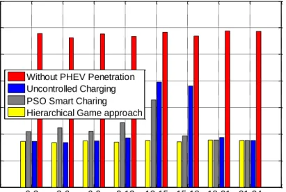
Table 3.2 gives the peak load of the system with different control strategies and penetration level. It shows that the ESPSO approach can effectively reduce the peak load. So for a fixed transformer power capacity in a residential distribution system, the proposed ESPSO approach can integrate more PHEVs into the system without overloading the transformer.

Table 3. 2 Peak Load of Different Control Strategies at Different PHEV Penetration Level (kW)

10% 20% 50% 100%

Uncontrolled Charging 395 432 524 686

PSO Smart Charging 372 372 394 452

(53)

4.

A Game-theoretic Framework for Vehicle-to-Grid

Frequency Regulation

Introduction

4.1

Various frameworks and algorithms have been proposed to apply V2G in frequency regulation [40]-[49]. In [40], the possibility for PHEVs to serve as primary frequency response unit is studied. PHEVs are used as supplementary LFC devices in [41]-[43]. Reference [44] applies particle swarm optimization and robust control t