Use of Principle of Contra Gradience for Developing Flexibility Matrix

(1)

Use of Principle of Contra-Gradience for Developing Flexibility Matrix

Vasudha Chendake

1

_{, Jayant Patankar}

2

1 _{Assistant Professor, Applied Mechanics Department, Walchand College of Engineering, Maharashtra, India} 2_{Professor, Applied Mechanics Department, Walchand College of Engineering, Maharashtra, India} ---***---Abstract - Flexibility method and stiffness method are the

two basic matrix methods of structural analysis. Linear simultaneous equations written in matrix form are always easy to solve. Also when computers are used, matrix algebra is very convenient.

When static degree of indeterminacy is less than the kinematic degree of indeterminacy, flexibility method is advantageous in structural analysis. The final step in flexibility method is to develop total structural flexibility matrix. The new approach to develop total structural flexibility matrix, requires force– deformation relation, transformation matrix and principal of Contra-gradience. Subsequently compatibility equations are required to get the value of unknown redundants. This new approach while using flexibility method is useful because simple matrix multiplications are required as well as order of the matrices does not become very large.

The application of this new approach to flexibility method is illustrated by solving few problems of structural analysis. MATLAB software is used to do matrix calculations. The results obtained by this new approach are compared with STAAD Pro results.

Key Words: Principle of Contra-gradience, MATLAB, STAAD Pro.v8i, Flexibility matrix

1.INTRODUCTION

In the flexibility method, the primary structure is the released form, where unknown actions have been released. The primary unknowns are the released unknown actions. A significant feature of the method is that the analyst has a choice in the selection of the action to be released. Flexibility coefficients giving the deformation values due to unit action applied in the direction of primary unknowns are used in the new approach of flexibility method along with force and deformation transformation technique. And those flexibility coefficients can be developed by using different methods of structural analysis for example unit load method, theorem of three moments, slope deflection equations.

This new method is used when static degree of indeterminacy is less than kinematic degree of indeterminacy. And order of matrix required in this new method is equal to static degree of indeterminacy. So order of matrices does not become very large which will occupy less memory of computer if program is made by using this new approach of flexibility method. The need of developing

computer program based of flexibility method is increased because the procedure of the direct stiffness method is so mechanical that it risks being used without much understanding of the structural behaviours.

Matrix algebra required in new approach of flexibility method is also very simple. So the time required for manual calculations can be reduced by using MATLAB software.

1.1Principle of Contra-gradience

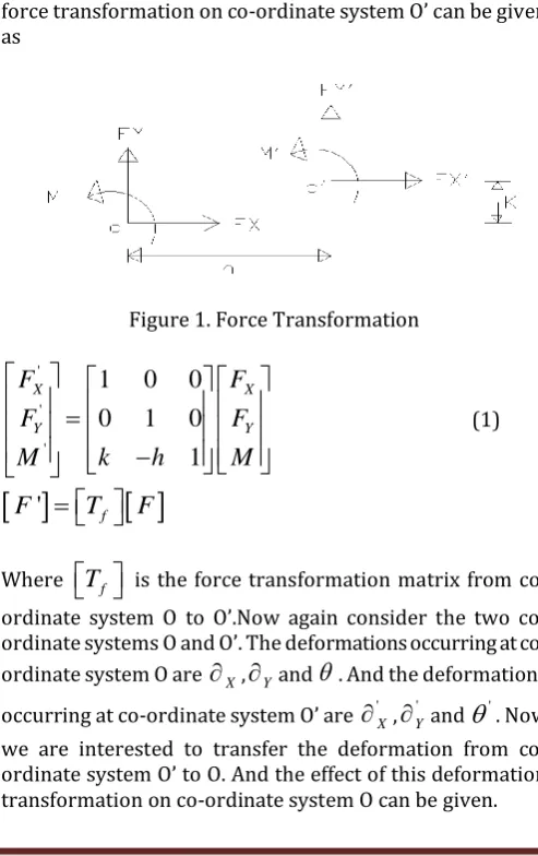
[image:1.595.308.555.388.780.2]

Consider the two co-ordinate systems O and O’ as shown in fig 1. The forces acting at co-ordinate system O are

F

_X ,

F

_Y and M and the forces acting at co-ordinate system O’ are

'

X

F

, '

Y

F

and '

M

. Here we are interested to transfer the

forces from co-ordinate system O to O’. And the effect of this force transformation on co-ordinate system O’ can be given as

Figure 1. Force Transformation

' ' '

1

0

1

0

1

X X

Y Y

F

M

k

h

M



 





 

_

 





 





 

_



 

_{ }



_





(1)

 

F

'

  

 

T

_f

 

F

Where

 

_{ }

T

_f is the force transformation matrix from ordinate system O to O’.Now again consider the two ordinate systems O and O’. The deformations occurring at co-ordinate system O are



_X,



_Yand  . And the deformations occurring at co-ordinate system O’ are '

X



, '

Y



and



'

(2)

[image:2.595.34.554.0.842.2]

' ' '

1

0

1

0

1

X X Y Y

k

h











 









_

 

_

_



_







 









 





 

  

(2)

    

 

T

_



'

Where

 

T

 is the deformation transformation matrix from

co-ordinate system O’ to O.

It is seen from equation (1) and (2) above

 

T f

T

_

  

 

Transpose of force transformation matrix from co-ordinate system A to B gives displacement transformation matrix from co-ordinate system B to A. This is known as Principle of Contra- gradience.

1.2 Nodal Deformation Method

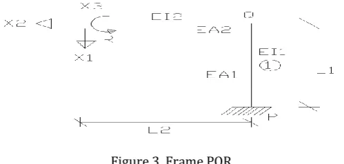
[image:2.595.37.287.540.659.2]

Figure 3 shows rigid jointed frame PQR with values of flexural rigidity (EI), axial force rigidity (EA) and length (L) for both members PQ and QR.

Figure 3. Frame PQR

Total deformation occurring at R is caused by mainly the deformations of both members PQ and QR. And for that flexibility coefficients are used which will give deformations due to the unit action. Total deformation can be given as

     

F



F

₁



F

₂

where

 

F

= Flexibility matrix for the frame PQR

 

F

1 = Deformation due to member PQ

 

F

2 =Deformation due to member QR

Figure 4. free body diagram

From the equilibrium of member QR,

1 1

2 2

3 2 3

0

1

0

1

0

1 Y

X

Y

X

Y

L

X

  

 



 

_







 

_

_





 

_

_



  

 



OR

 

Y

  



T

_QR



 

X

Where

 

Y

and

 

X

are the column matrices of the actions

Q and R respectively.



_

T

_QR



_

is the transformation matrix for the actions at Q from R. Hence

 

1

T

QR PQ QR

F





_

T

 

_

_

F

 

_{ }

T



_

(3)

 

3 2

2 2

0

3

2

0

2

QR

L

EI

L

F

EA

L

EI























_

_

 























Thus the flexibility matrix for the whole frame can be developed by using flexibility coefficients along with force and deformation transformation technique as well as principle of contra-gradience. Following examples will show the use of this new approach of flexibility method.

2. PROBLEMS AND ANALYSIS

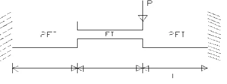
[image:3.595.43.274.359.445.2]

Example (1): The fixed beam shown in figure 5 where the length of each member is L and it is subjected to a concentrated force P. There is step variation of the flexural rigidity EI.

Figure 5. Fixed Beam

Static degree of indeterminacy = 2

The reaction R and moment M at fixed end D are considered as redundant as shown in figure 6.

Figure 6. Free body diagram of fixed beam

where,

By solving above equation, we will get

Compatibility condition at the point D is given by,

Calculations - solving manually,

In Example 1:

Put L= 3 m & point load P = 10 kN

By solving manually, results obtained are as follows

R = 7.5 kN M = -15 kN m

 CALCULATIONS -BY SOFTWARE (STAAD PRO) APPROACH:

(4)

Table- 1. STAAD PRO RESULT

 Calculations –by Using MATLAB SOFTWARE MATLAB INPUT

MATLAB OUTPUT

From above results, manual results are exactly matching with STAAD PRO results and MATLAB software can be used effectively for calculations.

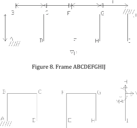
[image:4.595.39.574.100.842.2]

Example (2): A rigid jointed frame ABCDEFGHIJ is shown in figure 8. The flexural rigidity EI is uniform for the whole frame. Each element is of the same length L. The frame is subjected to a concentrated force P at the intermediate point E.

Figure 8. Frame ABCDEFGHIJ

Thus

By solving manually,

Horiz ontal

Vertical Horizont al

Moment kNm

Node Load _case Fx kN Fy kN Fz kN Mx My Mz

3 P = 10 _kN 0.000 7.495 0.000 0.000 0.00 14.986

4 P = 10 _kN 0.000 2.505 0.000 0.000 0.00 7.535

Figure 9. Free Body Diagram

[image:4.595.318.549.206.422.2]

(5)

The compatibility condition at the end J is written as

Yielding the answer

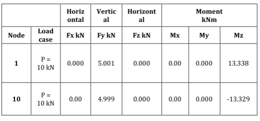
Put L= 3 m & point load P = 10 kN.

By solving manually, results obtained are as follows V = 0 kN,

H = 5 kN M = 13.33 kN m

[image:5.595.43.280.382.455.2]

CALCULATIONS: BY SOFTWARE (STAAD Pro) APPROACH

Figure 10. STAAD Pro MODEL OF 9 MEMBER FRAME

Table -2 STAAD Pro RESULTS

Horiz

ontal Vertical Horizontal Moment kNm

Node Load _case Fx kN Fy kN Fz kN Mx My Mz

1 _{10 kN}P = 0.000 5.001 0.000 0.00 0.000 13.338

10 _{10 kN}P = 0.00 4.999 0.000 0.00 0.000 -13.329

3. CONCLUSIONS

The application of new approach of flexibility method is shown here by solving examples. Results obtained from manual calculations are exactly matching with software results. So flexibility coefficients of individual members along with force and deformation transformation technique and principle of Contra-gradience can be used to develop the flexibility matrix for the whole structure. Also MATLAB software can be used to do mathematical calculations.

REFERENCES

[1] B.Parikh, J. Patankar, and V.Inamdar, “Use of nodal deformations in flexibility method”, International Conference on “The Concrete Future” Kuala Lumpur, Malaysia,25-26 February 1992.

[2] R. Mohankar, P.Thakare, P.Bhagwatand P. Dhoke, “Comparative Study of Beam by Flexibility Method & Slope Deflection Method.”,International Journal of Science, Engineering and Technology Research (IJSETR), vol. 5, Issue 2, February 2016.

[3] John L. Meek, “ Matrix Structural Analysis”, McGraw-Hill book company,1971.

[4] Devdas Menon, “Structural Analysis” eighth edition Published by Pearson Prentice Hall Pearson Education, Inc.2008.

[5] C.S. Reddy, “Basic Structural Analysis”, Tata McGraw Hill Education Private Limited, New Delhi,2011.

[6] R.C. Hibbeler, “Structural analysis”, eighth edition Published by Pearson Prentice Hall Pearson Education, Inc.2012.

[7] Victor E. Saouma, “Matrix Structural Analysis with an Introduction to Finite Elements”,Dept. of Civil Environmental and Architectural Engineering, University of Colorado, Boulder, CO 80309-0428, 1999.

[image:5.595.32.292.525.646.2]