Development, Optimization, and Analysis of Cellular Automaton Algorithms to Solve Stochastic Partial Differential Equations

© 2017, IRJET | Impact Factor value: 6.171 | ISO 9001:2008 Certified Journal

| Page 1466

Development, optimization, and analysis of cellular automaton

algorithms to solve stochastic partial differential equations

Ekesh Kumar

_{, Bryan Gorman}

_{, Jeffrey Brown}

1,3Research mentee, Johns Hopkins University Applied Physics Lab; Laurel MD, United States 2 _{Research mentor, Johns Hopkins University Applied Physics Lab, Laurel MD, United States}

---***---Abstract –

performance and optimization of cellular automaton algorithms that can approximate stochastic partial differential equations (SPDEs). We propose a central finite-difference scheme for an SPDE that exhibits angular diffusive properties and a velocity constraint with a stochastic process satisfying the Markov property. We show, using a non-Markovian Monte Carlo algorithm, that the probability distribution computed by the finite-difference method is moderately accurate. While performing this convergence analysis, we can establish a relationship between two variables that likely links back to a foundational finding of stochastic analysis, namely the dW2 _{= dt}2 _relationship

between the Wiener process and time. Finally, we analyze previously published work that can benefit from our findings, and we discuss possible courses of actions that can be taken to advance this research even further.

Key Words: Stochastic Partial Differential Equation, Cellular Automaton, Algorithms, Numerical Analysis

1.INTRODUCTION

In the modern age of information complexity, the use of stochastic processes to model random phenomena has significantly increased. With the increasing popularity of stochastic processes in various fields including quantum field theory, statistical mechanics, and stock market fluctuations, stochastic calculus has attracted much attention, especially in recent years. An example of such equations used to model such random processes are the stochastic Liouville-von Neumann equation, used to describe energy transfer dynamics, and the stochastic Navier-Stokes equations, used to describe hydrodynamic fluctuations.

Einstein and Smoluchowski are prominent figures known for their foundational work on stochastic differential equations (SDEs) through their explanations of the kinetic theory of matter and Brownian motion. Stochastic partial differential equations (SPDEs) allow for the extension of the capabilities of SDEs to phenomena in greater dimensions. It has been discovered that even the most fundamental stochastic processes are mathematically complex; thus, they require their own rules for calculus.

The most common interpretations of stochastic calculi have been generalized by Itô and Stratonovich.

Due to the mathematically complex nature of stochastic processes, there are limited cases in which SPDEs can be solved analytically. Moreover, contemporary numerical algorithms are not optimal for deriving an exact form of their solutions either; so, we are compelled to seek an accurate and efficient method to better approximate these equations. A newly developing method to approximate the solution of SPDEs involves the use of cellular automata. The utilization of cellular automata allows one to represent the diffusion processes associated with SPDEs in a discretized n-dimensional mesh-based grid, like a dynamical system. The concept of cellular automaton was developed by Neumann and Ulmann in the 1940s. This topic developed throughout the 20th and 21st centuries through the popularization of various models, such as Conway’s Game

of Life. In 2002, Wolfram published A New Kind of Science

[2] in which he asserts that the use of cellular automaton has a multitude of applications. The work discussed in this paper is a continuation on this foundational work.

The goal of this paper is to develop numerical approximation algorithms for solving SPDEs efficiently and accurately. This paper considers the development and optimization of novel cellular automaton numerical approximation methods of a stochastic partial differential equation. The SPDE that is discussed in this paper exhibits basic angular diffusive properties with a velocity constraint. However, the methods described in this paper can be readily applied to approximate other SPDEs.

© 2017, IRJET | Impact Factor value: 6.171 | ISO 9001:2008 Certified Journal

| Page 1467

,

where p is the probability density function, t is time in hours, x and y are directions in a standard Cartesian plane in nautical miles, and φ is a stochastic variable corresponding to the angular position of the subject. This equation was derived around the Wiener process.

The stochastic process in these equations satisfy the Markov property, meaning that the conditional probability distribution of future states is dependent only on the present state; states prior to the present one have no impact on future states.

1.1

Finite-Difference Method

The goal is to approximate solutions to SPDEs that have boundary conditions on the edges of their domains, which, in general, is a very difficult task. Finite-difference methods (FDMs) are numerical methods used to solve differential equations by replacing their derivatives by finite-difference approximations. These approximations provide a system of equations that can be solved using computation software much easier instead of the differential equation. There are three forms of finite-difference methods that are most commonly considered: forward, backward, and central. As their names suggest, forward and backward differences predict derivatives based on points ahead and behind the desired derivative, respectively. Central differences, which average forward and backward differences, are obviously better approximations of derivatives. As defined by LeVeque [3], the center difference used to approximate the partial derivative of a smooth, differentiable, one variable function u(x) at a point x is given by

D0u(x) ( ) ( )

This scheme can be expanded to higher-ordered differential equations. The error of the center difference is proportional to ∆x2 _{, which is very small relative to the} forward and backward difference methods that have an error roughly proportional to ∆x.

A three-dimensional FDM function was implemented to model the behavior of equation (1) with y as the first dimension, x as the second dimension, and φ as the third dimension. The algorithm required velocity and standard deviation after one hour of motion as inputs, while range resolution and course resolution could be provided as optional inputs. The pseudocode for the implemented algorithm is as follows:

Algorithm 1: Finite-Difference Method function FDM

 Initialize diffusion constant and other variables

 Set up mesh-grid as a two-dimensional array

 Apply boundary conditions to mesh-grid

 Find the difference between each cell in the positive

x-direction

 Multiply the differences by the sine of the angle in a given slice of the tensor

 Add the difference to mesh with mass distributions

 Repeat for variable y

 for all n:

 Sum the central finite-difference in the φ

dimension

 end loop

 Add difference original probability mass

distribution mesh

 return probability distribution

Data was collected for several values of n while holding different values of velocity and standard deviation at a constant value. The probability distributions collected from the FDM were exported to spreadsheets, where they were analyzed for trends

1.2 Monte Carlo Integration

A Monte Carlo method is a computational algorithm that employs large-scale random sampling to determine a numerical approximation of a stochastic process. The key concept behind Monte Carlo integration is to utilize the Law of Large Numbers, which states that the average of values computed through random sampling will eventually converge to their corresponding probabilities. For example, suppose one is interested in approximating a variable y that can be expressed as

∫ ( ) ( )

where X is a random variable with probability density fx, g is a function, and x1, x2 . . . x3 are random numbers distributed according to the density fx. Then, the average

∑ (

)

approximates y.

© 2017, IRJET | Impact Factor value: 6.171 | ISO 9001:2008 Certified Journal

| Page 1468

we were to double the precision of the Monte Carlo approximation, the number of simulations would need to be quadrupled.

The motive behind developing a Monte Carlo algorithm was to implement a reliable method that would allow for a rough comparison of other approximation results. The Monte Carlo algorithm that was constructed to achieve this goal was non-Markovian. The pseudocode of the algorithm is shown:

Algorithm 2:Monte Carlo Integration function Monte_Carlo

 Initialize variables and constants

 for each n

 Generate a vector full of random values of φ

 Add rsin(φ) to x data

 Add rcos(φ) to y data

 Collect and normalize positions to a probability mass distribution

 end loop



Each call to the function simulates 10,000,000 trials at a constant speed in intervals of one time step at a time. Data was collected holding these values constant, with varying

values of maxAngle. This provides a rough estimate of how

the probability distribution should look like.

2. HEADING 2

With the data collected from stages I and II, various tests were conducted to determine whether there was a large correlation between the two computed probability densities. This allowed us to verify whether the implemented numerical methods had been reasonably accurate.

In addition to finding trends between the two numerical approximations, we sought a method of approximating the two one-dimensional arrays created in the initial two stages. This was accomplished by performing a regression analysis on the two data sets and finding an equation that accurately represents their trend.

Through Stage I, we gained multitudinous amounts of data depicting probability distributions recorded at different loop values. The probability distributions were stored in spreadsheets as two-dimensional arrays. The largest probability value in each distribution was recorded into a separate one-dimensional array. In addition, the FDM provided more information regarding the behavior of the SPDE that was being approximated. Through the

collected data, it was found that much of the probability mass was swelling to the sides. With every time step taken, this recurring trend spread and accumulated increasingly larger amounts of probability mass, especially on the sides of the two-dimensional array. This was a direct consequence of the wave-like process that the FDM employed.

Stage II reinforced much of what was found in the initial stage. Even more probability distributions were collected through this method. In addition, since the Monte Carlo algorithm allowed its user to input the maximum angle of deviation as a parameter. Another one-dimensional array was created to hold the values of loops corresponding to this angle

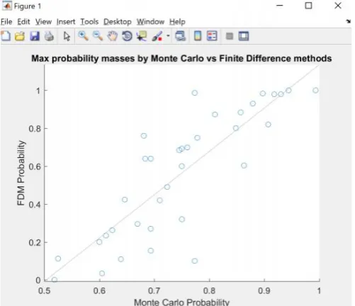
The plot exhibits the trend between the greatest probability mass in the distributions collected by the FDM and Monte Carlo algorithms in the first two stages. The linear regression, representing close to 500, 000, 000 Monte Carlo simulations, demonstrates that the FDM implemented in Stage I was accurate; the two computation methods were found to have a Pearson correlation coefficient of r = 0.84

Figure 1: Plot comparing probability mass value computed by two different numerical algorithms show a

strong positive trend

© 2017, IRJET | Impact Factor value: 6.171 | ISO 9001:2008 Certified Journal

| Page 1469

allowed us to estimate one of the variables given the other. Next, a polynomial interpolation script was employed to compute angle deviation values to fill in the gaps that were present between previously collected data points. The benefit of finding a function to model this relationship was that it was continuous and differentiable everywhere, which allowed for better analysis. In addition, the interpolation script was tested against the data that had already been collected, which revealed that the polynomial had a low margin of error. As shown in Figure 2, the margin of error for the computed values of angle deviation was small even for large angle.

Figure 2: Plot comparing the actual maximum angle of deviation versus the maximum angle of deviation computed via polynomial interpolation. Results show a

relatively small margin of error, even for large angles.

3. CONCLUSIONS

The expected outcome of this research was to produce a numerical algorithm that could compute SPDEs as close to the analytical solution as possible without exceeding a

computationally practical runtime. With the

implementation of a Monte Carlo algorithm, we could gain information on whether the FDM had some accuracy. We found that there was a moderately strong positive trend between the FDM and Monte Carlo approximations, which infers promise in this method. However, since a non-Markovian Monte Carlo algorithm was used to approximate a stochastic process that satisfies the Markov property, even the Monte Carlo approximation is less than optimal. The implication of this discrepancy is that the FDM could be slightly more accurate or slightly less accurate than what was predicted.

During the process of creating an accurate approximation, it was important for the numerical

algorithms to take boundary conditions into

consideration. Using Neumann and Symmetric boundary conditions, we could specify a region for the SPDE to be solved, which allowed for unique solutions. This was a step that was not present in some previous work [5], which led to an increased error in their approximations.

In investigating these phenomena, we also found an inverse-square relationship between the number of loops required to model the second-order diffusive term and the angle that it seemed to correspond to. In the opinion of this investigation, we believe that the inverse-square relation is evidence of a deep pattern in stochastic

analysis, particularly, the well-known dW2 _{= dt}

relationship [6], where W and t are the Wiener process and time, respectively

These findings cannot be referenced in other journals because of a lack of published material on the numerical analysis of SPDEs. While Bućkova et. al.[5] credit finite-differences as a viable tool to solve SPDEs, the research does not specifically include an implementation or analysis of the method. In addition, an exhaustive literature review could not find any work that was able to associate an inverse-square relationship of an SPDE to the foundational stochastic differential.

These conclusions are also capable of enhancing the findings of previous work. For instance, Giles et. al. [8] develops a differing numerical method of solving SPDEs, but states, “For the initial-boundary value problem . . . an efficient numerical method is needed.” This is an issue that the FDM mitigates to a large extent by taking Neumann and Symmetric boundary conditions into consideration. Similarly, Deb et. al. [9] could benefit from this work by gathering additional data from our numerical methods to compare to their approaches. Several other approaches of research can also be expanded upon with this method of approximation; the technique allows us to minimize the margin of error by considering all boundary conditions, which reduces the number of “after-adjustments” needed.

© 2017, IRJET | Impact Factor value: 6.171 | ISO 9001:2008 Certified Journal

| Page 1470

computational problem.

Essentially, through a systematic approach that iteratively collected large amounts of data, this research enabled us to attain a moderately accurate approximation of SPDEs. Moreover, this work could reproduce the

well-known dW2 _{= dt inverse square relationship in a nontrivial}

manner. Consequently, this work will allow future research in the fields of numerical and stochastic analysis to make use of the inverse square that can be found in the variables of the SPDE that they are working with. Because of this work, models involving stochastic processes will improve, which can be beneficial in most scientific fields.

The results that are detailed in this report are only supported by the results described in this paper since there is a limited amount of published pertinent literature analyzing the use of FDMs in approximating SPDEs. In addition, there is a limitation on what can be achieved computationally as the approximations are still inherently random.

Despite the success we have had with these methods, the methods used in this paper are not infallible. Much of the testing performed in this paper relied on random sampling that, due to computational limitations, could potentially be less than optimal. Furthermore, the algorithms that were being utilized to collect data did so in a wave-like diffusion manner. It was found that this technique of organizing collected data yielded a swelling of probability mass to the sides of the two-dimensional array, which led to under approximations of the greatest probability mass in long-term testing. In addition, data was not analyzed for long-term scenarios, in which it is likely that the algorithms utilized in this report will produce inaccurate results.

To improve this research, it is essential to implement a method of redistributing the probability mass that is accumulating to the sides of the two-dimensional array. One possible approach to resolve this issue would be to construct a Markov Chain Monte Carlo algorithm that makes decisions of reallocating probability mass on the basis of its current state. It would also be beneficial to develop newer numerical methods that allow us to investigate the behavior of SPDEs from different perspectives.

Earlier in this research, different methodologies that relied on primarily physics-based principles were attempted rather than mostly mathematical methods. One approach was to treat the behavior of the SPDE as a closed system. The fact that energy is conserved, by the First Law of Thermodynamics, would allow us to repeatedly recalculate the total energy of the system using

Hamiltonians or other energy functions. In summary, the allocation of the probability mass could be based on the motion of the “ship.” A problem that arose from this approach, however, was that it did not consider the SPDE’s boundary conditions or the computational difficulty associated with persistently calculating equations that govern such behavior.

Through this research, we could address some of the deficiencies that other approximation methods faced. The future of this research lies in the optimization of the numerical methods along with the development of newer methods. It is also a necessity to develop a more sustainable method of testing the accuracy of approximations, specifically one that satisfies the Markov process. These progressions will help completely automate the process of solving these equations, which will be invaluable to all who make use of SPDEs

REFERENCES

[1] Gardiner, C. W. (2002). Handbook of stochastic

methods for physics, chemistry and the natural sciences (Vol. 2). Berlin: Springer.

[2] Wolfram, S. (2002). A New Kind of Science.

Champaign, IL: Wolfram Media

[3] LeVeque, R. J. (2007). Finite difference methods for

ordinary and partial differential equations: steady-state and time-dependent problems. Philadelphia, PA: Society for Industrial and Applied Mathematics.

[4] Burden, R. L., Faires, J. D. (2011). Numerical analysis

(9th ed.). Boston, MA: Brooks/Cole, Cengage Learning.

[5] Herzog, F. (2013). Brownian Motion and Poisson

Process. Ethz Special Interest Topics

[6] Buˇckov´a, Zuzana Stehl´ıkov´a, Be´ata Sevˇcoviˇc,

Daniel. (2016). Numerical and ˇ analytical methods for bond pricing in short rate convergence models of interest rates. (p. 6).

[7] . Belavkin, R. V. (2017). Lecture 7: Ito differentiation

rule. Retrieved from Middlesex University Pricing and Stochastic Calculus

[8] Giles, M. B., Reisinger, C. (2012). Stochastic Finite

Differences and Multilevel Monte Carlo for a Class of SPDEs in Finance (Vol 3). Society for Industrial and Applied Mathematics

[9] Deb, M. K., Babuˇska, I. M., Oden, J. T. (2000). Solution

of stochastic partial differential equations using Galerkin finite element techniques