A NEW SOFT SET BASED PRUNING ALGORITHM FOR ENSEMBLE METHOD

(1)

ISSN: 1992-8645 www.jatit.org E-ISSN: 1817-3195

INFORMATION TECHNOLOGY FOR NUMERICAL

SIMULATION OF VISCOUS INCOMPRESSIBLE FLOW IN

BICONNECTED DOMAINS

1_{NURLAN TEMIRBEKOV,}2_{SAYA TOKANOVA,}2_{YERZHAN MALGAZHDAROV}

1

Kazakhstan Engineering Technological University, Almaty, Kazakhstan

2

S. Amanzholov East Kazakhstan State University, Ust-Kamenogorsk, Kazakhstan

ABSTRACT

This paper analyzes the method of supplemented domains for the numerical simulation of viscous incompressible flow in the complex geometrical domain. The problem is considered in a discrete defined biconnected domain with the curved boundary. The spline interpolation of curved boundary is conducted. The Navier-Stokes equations for viscous incompressible fluid are selected for the numerical simulation. A stable finite-difference scheme and an algorithm of numerical implementation are developed. The numerical results are obtained with different numbers of grid nodes.

Keywords: Navier-Stokes Equations, Viscous Incompressible Fluid, Numerical Simulation, Numerical Experiment, Stream Function, Method Of Supplemented Domains, Cube Spline Interpolation, Curvilinear Biconnected Domain.

1. INTRODUCTION

Many problems of hydrodynamics, hydromechanics, hydraulics, acoustics, circulatory physiology, organization of technological processes due to a moderate speed of the medium, as well as phenomena observed in the atmosphere and ocean can be studied within a viscous incompressible fluid.

At the present time, applied scientists have different problems, a thorough research of which can be carried out in most cases only by computational experiment (CE) or through a carefully staged physical experiment. However, the phenomena of practical interest and technological processes either cannot be fully physically simulated or the costs of such experiments are too high.

An effective method for studying the dynamics of a homogeneous fluid flow is numerical simulation, which allows analyzing the flow in a wide range of changes in key parameters using computational experiments on a computer. Over the last years, questions of numerical simulation of the Navier-Stokes equations for incompressible fluid attracted much attention of mathematicians and engineers.

Tasks of practical interest, as a rule, are characterized by multidimensionality, nonstationarity, nonlinearity, the presence of free

boundaries and boundary layers and are described by the Navier-Stokes equations. The nonlinearity of the Navier-Stokes equations and the presence of a small parameter in the highest derivatives (especially in high Reynolds numbers) create serious difficulties both during their desk study (it is possible only for the model equations or specific tasks) and the numerical solution of these equations with the help of a computer.

Recently, due to the rapid development of computer technology and computational mathematics the role of renewable energy for the simulation of complex nonlinear hydrodynamic problems has significantly increased. The basic principles underlying renewable energy are described in sufficient detail in the works by N.S. Bakhvalova, O.M. Belotserkovskii, G.I. Marchuk, A.A. Samarskii, P. Roach, N.N. Yanenko, their colleagues and students.

The technological cycle of renewable energy includes the following main stages:

1) the construction of a physical model - at this stage there is the clarification of the basic physical processes and mechanisms inherent to the studied phenomenon or process;

(2)

ISSN: 1992-8645 www.jatit.org E-ISSN: 1817-3195 equations with the necessary initial and boundary

conditions;

3) then the important step in the technological cycle is the construction of a computational algorithm that includes two main points: the construction of a discrete mathematical model, i.e. the approximation of the original difference problem, and the development of an efficient method for solving the difference problem;

4) this is followed by writing, creating and debugging a program on the computer;

5) then a series of test calculations for judging the correctness and accuracy of the algorithm and the program are carried out;

6) finally, there are the numerical solution of the initial mathematical problem.

Finally, a comparison of the results with the experimental data and calculations of other authors is carried out, on the basis of which a conclusion about the adequacy of the selected physical model of the phenomenon under investigation is made. It should be taken into account that the level of physical and mathematical models, the algorithm and its precision, as well as configuration, performance, and memory of computers should be mutually balanced.

During the development of a physical model, it is necessary, first of all, to take into account the main features of the phenomenon and to try to get adequate results on the model as simple as possible, reflecting the essence of the phenomenon.

Thus, the main mechanism in separated flows of viscous fluid is the mechanism, conditioned by the presence of liquid adhesion to the solid surface of the body. Errors in the simulation of this mechanism having a molecular nature can significantly affect the results obtained. Thus, in the simulation of separated flows, particular attention should be paid to the adequate representation of flow near the surface of the body, which is especially important with an increase in the Reynolds number (with a decrease in the thickness of the boundary layer). Moreover, in the range of the critical Reynolds numbers, when there is a loss of stability of the laminar boundary layer, and there are large-scale vortex formations - stains inside the boundary layer, it is necessary to correctly reproduce the birth and dynamics of these formations, i.e. for the calculation of such conditions it is necessary to use finite-difference grids with an appropriate resolution.

On the other hand, a flow in the near wake of the body of a finite size for both laminar and turbulent flow conditions is characterized by the presence of large-scale vortices, the dimensions of which are comparable with the linear dimensions of the body, and therefore, the resolving power of a finite difference grid can herein be substantially weakened. Of course, there may be mistakes in the approximation of the dissipative mechanism of such vortices, but the main features of the phenomenon, including a number of quantitative characteristics, are being reproduced quite accurately.

Most existing methods for solving the Navier-Stokes equations do not allow to get reliable results in the study of properties of the viscous fluid of the bodies with complex shapes (ea. in determining the aerodynamic characteristics of modern aircraft and submarines), especially for large Reynolds numbers and for turbulent flow conditions. Rather precise quantitative data, comparable to a physical experiment, were obtained mainly for laminar flow conditions in the two-dimensional stationary tasks.

Mathematical modeling of such complex flows as spatial separated flows, especially in high Reynolds numbers, flows with a free surface, flows of stratified fluid density and substantially three-dimensional flows in technological devices and industrial buildings for special purposes, imposes a number of requirements for the applied and developed methods of solving equations describing these trends.

These requirements include a high order of the approximation of finite difference schemes - second or higher; a minimum circuit dissipation and dispersion; the performance in a wide range of tested parameters (Reynolds numbers, and others) and the monotony. The latter feature is particularly important for simulation of flows with areas of large gradients of hydrodynamic parameters and calculations with a free surface, as well as flows of stratified fluid.

Development of effective numerical methods as well as calculation of considerably nonlinear flows of incompressible fluid with their use is rather relevant.

(3)

ISSN: 1992-8645 www.jatit.org E-ISSN: 1817-3195 Navier-Stokes equations have become one of the

first objects using the numeric methods. Many problems of viscous flow dynamics, for example the problem of numerical research of flows under high under and over critical numbers of Reynolds are not solved till nowadays and should be solved with great emphasis.

Works of a famous French mathematician Roger Temam are dedicated to rather considerable exposition of questions of theory and particularly calculation aspects of viscous incompressible fluid, the questions of existence, uniqueness and regularity properties of boundary value problems for the Navier-Stokes equations are considered [1, 2]; the most general and special methods used for study of different kinds of flows are offered in works of K. Fletcher [3].

Numeric methods of the boundary value problem of mathematical physics in complex domains were considered in many works of foreign and national scientists: Baldybek [4], Vabishchevich [1], Mukhametzhanov, Otel’bayev and Smagulov [5], Smagulov and Otel'bayev [6], Danayev [7], Smagulov, Danayev and Temirbekov [8].

The Navier-Stokes equations are of the evolutionary nature. For the first time, this idea was put forward in the work [9]. Main elements of construction technology of adaptive differential grids in bidimensional and tridimensional domains, and basis of design methods of curvilinear grids are provided in the works [10] and [11]-[14].

Numerical simulation of established fluid flows within the curved boundaries is conducted in most papers on the basis of the viscous incompressible fluid model [15]. The algorithms based on the Navier-Stokes equations using the finite-difference method are widely distributed.

Currently, there is a large number of numerical methods solving the Navier-Stokes equations that describe the flow of an incompressible viscous fluid. Most of these methods have been developed with reference to the system of equations written with respect to the stream function ψ and the vortex ω in the natural variables (

( )

ur,p - a system or primitive equations).

The common disadvantage of these methods is the use of some form of boundary conditions for the vortex in the variables

(

ψ,ω

)

and for pressure in

the variables

( )

ur,p on a solid body surface, which is absent in the physical statement of the task. An additional iteration process associated with the

specified boundary conditions for the vortex limits the rate of convergence of numerical algorithms. It is obvious that the difference scheme, which allows to calculate the flow of a viscous incompressible fluid without the use of the boundary conditions for the vortex on a solid surface, under all other equal conditions is more effective.

This paper considers the algorithm of numerical realization of the Navier-Stokes equations for a viscous incompressible fluid in the variables

(

ur,ψ

)

, which will allow to get rid of these problems.

At the present time, it is increasingly required to solve problems in complex areas with complex geometry. There are some methods of numerical solution of boundary value problems in complex geometrical domains as the curvilinear grids method and the fictitious domains method [16]. Use of the curvilinear grids method requires transformation of an equation into curvilinear coordinates which leads to more complicated equations than the original ones. Moreover, diverse requirements imposed on the difference grid, make building curvilinear grids a complex mathematical problem.

The fictitious domains method in its traditional formulation is simple to use and is simply implemented. But its disadvantage is loss of accuracy because of presence of a small parameter in subsidiary equations which leads to ill-conditioning of difference equations.

In this work, the numerical simulation of viscous incompressible fluid flow in the discrete biconnected domain using the method of supplemented domains is studied. The algorithm of numerical implementation of the method offered in the work [4], in which there is no small parameter.

2. FORMULATION OF THE PROBLEM

We consider the Navier-Stokes equations in a two-dimensional domain Ω_{with a boundary}∂Ω:

(

u

)

u p u f

t

ur _r _r _r r

+ ∆ = ∇ + ∇ ⋅ + ∂ ∂

µ (1)

0

= ⋅

∇ ur ₍₂₎

with initial and boundary conditions

( )

x y u

ur= r₀ , when

( )

x,y ∈Ω, t=0

(

x y t

)

(4)

ISSN: 1992-8645 www.jatit.org E-ISSN: 1817-3195 where х,у are Cartesian coordinates, t is time,

u

r

is velocity field, p is deflection of pressure, µ is viscosity coefficient.

3. COMPUTATIONAL ALGORITHM

The initial system of equations (1)-(2) is written with respect to an arbitrary curvilinear coordinate system. The pressure and speed pattern concordance was executed with the help of the fictitious domains method modified for calculation of the problem. The structured grids were used for creation of the discrete analogue of initial equations about a figure of complex geometry as basis equations. The multiblock computational technologies were used in the biconnected domain. Such approach has allowed to develop a common methodology for calculation the viscous fluid flow in biconnected domains.

The system of initial equations was integrated numerically using the method of supplemented domains. Derivatives in the viscous terms are approximated by central-difference scheme of second order.

The whole considered domain of continuous variation of the argument is replaced by a discrete change domain, i.e. we introduce the following grid:

( )

(

)

; 2 1 , 1 1 , 2 2 2 , 1 1

1 _

    − = − = = = =

Ω j h

j y h i i x n l h n l h h . 2 , 1 , 1 ,

1n j n

i= =

(4)

The staggered grid pattern was used in the work where pressure and divergence are determined in nodes of difference grid, stream function is in the center of the difference cell, and velocity components are in the center of its bounds.

[image:4.612.311.529.451.695.2]

The use of the staggered grids allows to join the velocity components in neighboring points and avoids the appearance of oscillations in the calculation of the pressure field (Fig. 1, where - component

u

, - component

ω

, - pressure).

Figure 1: Staggered Grid Pattern

The components of velocity, pressure and stream function are determined in the following points:

(

)

{

}

(

)

{

}

{

}

. 2 , 1 : ; 2 2 1 , 1 : ; 2 , 1 2 1 : jh j y ih i x p h j j y ih i x jh j y h i i x u = = − = = = − = υ

(

)

(

)

. 2 2 1 , 1 2 1 :     

 ₌ ₋ ₌ _j₋ _h

j y h i i x ψ

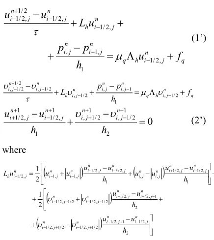
Difference analogs of (1), (2) are written in the form: q n j i h q n j i n j i n j i h n j i n j i

f

u

h

p

u

L

u

+

Λ

=

−

+

−

− − − − + − , 2 / 1 1 , 1 , , 2 / 1 , 2 / 1 2 / 1 , 2 / 1

µ

τ

(1’) q n j i h q n j i n j i n j i h n j i n j i f h p p

L + − = Λ +

+ − − − − − + − 2 / 1 , 1 1 , , 2 / 1 , 2 / 1 , 2 / 1 2 / 1 , υ µ υ τ υ υ 0 2 1 2 / 1 , 1 2 / 1 , 1 1 , 2 / 1 1 , 2 /

1 − ₊ − ₌

+ − + + + − + + h h u

u inj

n j i n j i n j

i

υ

_(2’)

(5)

(

)

(

)

(

)

(

)

        − − + − + + +     − − +     + − + = − + − − − − − − + − + − + − − − − − − − − 2 2 / 1 , 2 / 1 , , , 2 2 / 3 , 2 / 1 , 1 , 1 , 1 2 / 1 , 2 / 1 , 1 2 / 1 , 2 / 1 2 / 1 , 2 / 1 1 2 / 1 , 1 2 / 1 , 2 / 1 , 2 / 1 2 / 1 , 2 / 1 2 / 1 , 2 1 2 1 h h h u u h u u L n j i n j i n j i n j i n j i n j i n j i n j i n j i n j i n j i n j i n j i n j i n j i n j i n j i h υ υ υ υ υ υ υ υ υ υ υ υ υ     − − −     − + +         − − − = Λ − − − − − − + − + − − − − − + − 2 1 , 2 / 1 , 2 / 1 2 / 1 , 2 / 1 , 2 , 2 / 1 1 , 2 / 1 2 / 1 , 2 / 1 , 2 1 , 2 / 3 , 2 / 1 , 1 , 1 , 2 / 1 , 2 / 1 , , 1 , 2 / 1 1 1 h u u h u u h h u u h u u h u n j i n j i j i x n j i n j i j i y n j i n j i j i x n j i n j i j i x n j i h q µ µ µ µ µ . 1 1 2 2 / 3 , 2 / 1 , 1 , , 2 2 / 1 , 2 / 1 , , , 2 1 2 / 1 , 1 2 / 1 , 2 / 1 , 2 / 1 , 1 2 / 1 , 2 / 1 , 1 2 / 1 , 2 / 1 , 1 2 / 1 ,     − −     − + +     − −     − − = Λ − − − − + − − − − − − − + − + − h h h h h h n j i n j i j i y n j i n j i j i y n j i n j i j i x n j i n j i j i x n j i h q υ υ µ υ υ µ υ υ µ υ υ µ υ µ

We received the difference analogues of respective convectional and diffusion summands. The difference scheme taking into account a sign was used for the convectional summands, and the values of components are determined in the undetermined nodes by average-out. For example:

2 2 / 1 , 2 / 1 , , n j i n j i n j i − + +

=υ υ

υ .

Let us describe the algorithm for the numerical solution of the problem (1)-(3). We use the splitting technique on physical processes for the numerical implementation.

First of all, let us determine intermediate values of speed u=

( )

u,υ

r

, excluding pressure:

q n h q n h n n f u u L u u + Λ + − = − + r r r r µ τ 2 1

; (5)

Then, we determine a pressure field using intermediate values. In order to derive an equation for the pressure, we substitute the following expressions in (2’)

1 1 , 1 1 , 2 / 1 , 2 / 1 1 , 2 / 1 h p p u u n j i n j i n j i n j i + − + + − + − − −

= τ (6)

2 1 1 , 1 , 2 / 1 2 / 1 , 1 2 / 1 , h p p n j i n j i n j i n j i + − + + − + − − −

=υ τ

υ (7)

and obtain 2 2 / 1 2 / 1 , 2 / 1 2 / 1 , 1 2 / 1 , 2 / 1 2 / 1 , 2 / 1 2 2 1 1 , 1 , 1 1 , 2 1 1 , 1 1 , 1 ,

1 2 2

h h u u h p p p h p p p n j i n j i n j i n j i n j i n j i n j i n j i n j i n j i + − + + + − + + + − + + + + − + + + − + − = = + − + + −

υ

(8)

Speed components are calculated on a certain pressure field with the help of (6) and (7). The problem here is the absence of boundary conditions for pressure. We find values of the stream function related to the speed components on the second step instead of pressure field to avoid this problem by the following expressions [17]:

2 1 2 / 1 , 2 / 1 1 2 / 1 , 2 / 1 1 , 2 / 1 h u n j i n j i n j i + − − + + − + − −

=

ψ

, (9)

1 1 2 / 1 , 2 / 1 1 2 / 1 , 2 / 1 1 2 / 1 , h n j i n j i n j i + − − + − + + − − −

=

ψ

υ

. (10)

We have the following expressions to find values of the stream function

2 1 1 + + ₌ Λ n h n

h rot u

r

ψ

; (11)

where 2 2 1 2 / 3 , 2 / 1 1 2 / 1 , 2 / 1 1 2 / 1 , 2 / 1 2 1 1 2 / 1 , 2 / 3 1 2 / 1 , 2 / 1 1 2 / 1 , 2 / 1 1 2 2 h h n j i n j i n j i n j i n j i n j i n h + − − + − − + + − + − − + − − + − + + + − + + + − = Λ ψ ψ ψ ψ ψ ψ ψ 1 2 / 1 2 / 1 , 1 2 / 1 2 / 1 , 2 2 / 1 1 , 2 / 1 2 / 1 , 2 / 1 2 1 h h u u u rot n j i n j i n j i n j i n h + − − + − + − − + − + − − −

= υ υ

r

.

Using (9) and (10), we find the velocity field

1

+ n

u

r

.

The problems (5), (6), (7), (8) and (5), (9), (10), (11) are equivalent.

(6)

(

)

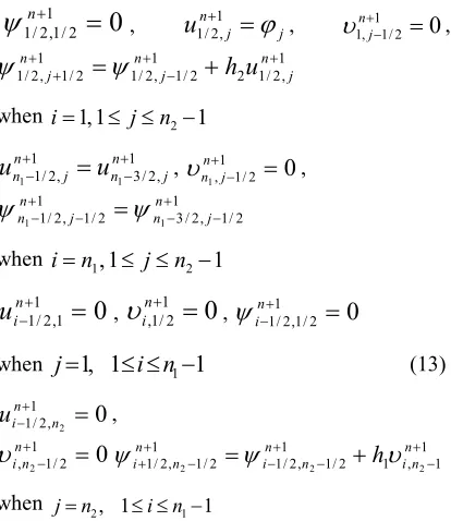
0 , 2 / 1 2 2 1 2 / 3 , 2 / 1 1 2 / 1 , 2 / 1 2 1 1 2 / 1 , 2 / 3 1 2 / 1 , 2 / 1 , 1 2 / 1 , 2 / 1 1 ψ θ ψ ψ ψ ψ θ ψ j i n h n j i n j i n j i n j i j i n j i u rot h h +     − + +     + + − = + + − − + + − + − − + − + + − − r (12) where     Ω Ω ∈ Ω ∈ = − − − − 2 1 2 / 1 , 2 / 1 0 2 / 1 , 2 / 1 , , , 1 , 0 j i j i j i ψ ψ θ , 0

ψ _{- stream function values on boundaries of the}

supplemented and fictitious domains. Let us suppose that the flow moves toward the direction of

x

_{as it is shown on Fig.2. Then, the boundary}

conditions are determined as follows:

0

1 2 / 1 , 2 / 1

=

+ n

ψ

,

u

n+1_j

=

ϕ

_j , 2 /

1 , 0

1 2 / 1 , 1 = + − n j

υ

, 1 , 2 / 1 2 1 2 / 1 , 2 / 1 1 2 / 1 , 2 / 1 + + − +

+

=

+

n j

n j n

j

ψ

h

u

ψ

when i=1,1≤ j≤n₂−1

1 , 2 / 3 1 , 2 / 1 ₁ 1 + − +

−

=

nn j

n j

n

u

, _,1₁_/₂ 0

1 = + − n j n

υ

, 1 2 / 1 , 2 / 3 1 2 / 1 , 2 / 1 1 1 + − − + − −

=

n j n n j n

ψ

when i=n₁,1≤ j≤n₂−1

0

1 1 , 2 / 1

=

+ − n i

u

,

υ

_in_,₁+_/1₂

=

0

, 1

0

2 / 1 , 2 / 1

=

+ − n i

ψ

when j=1, 1≤i≤n₁−1 (13)

0 1

, 2 /

1 2 =

+ − n n i u , 0 1 2 / 1

, 2 =

+ − n n i

υ

1 1 , 1 1 2 / 1 , 2 / 1 1 2 / 1 , 2 /

1 2 2 2

+ − + − − + − + = + n n i n n i n n

i

ψ

h

υ

ψ

when j=n₂, 1≤i≤n₁−1

Boundary conditions were calculated at the boundaries of the streamlined body as follows. Using a physical sense of the stream function in the fictitious domain Ω2, the values of stream function are considered as constant:

) (

5 .

0 1/21, 1/2

1 2 / 1 , 2 / 1 1 2 / 1 , 2 / 1 2 + − + + −

− = + n n

n n

j

i

ψ

(14) The methodical calculations were conducted using the offered method. Let us consider a curvilinear biconnected domain. We supplement the considered domain to a rectangle (Fig. 2) to apply the structured rectangular grids.

If the boundaries of the physical domain were set by the discrete set of points

( )

(

xi,f xi

)

,i=1,K,n,

[image:6.612.92.299.307.546.2]

the determination of grid nodes at the external and internal boundaries for provision of continuity and monotoneness of the boundary creates some difficulties, and it is often necessary to change a number of grid nodes by the numeric simulation.

Figure 2: Biconnected Discretely Defined Domain

The following cube spline interpolation [18] was used to provide continuity and monotoneness of the curvilinear boundary as well as automation of change in the number of grid nodes:

( )

(

)

(

)

2

(

)

3

6 2 i i i i i i i

i x x

d x x c x x b a x

s = + − + − + − (15)

The coefficients a_i,b_i,c_i,d_i are defined as follows:

( )

i i i i i i i i i i i i i i h c c d h a a h d h c b x f

a 1 1

2

, 6

2

, = − + − − = − −

= (16)

(

)

0 , 6 2 1 1 1 1 1 1 1 1 = =       − − − = + + + − + + + + + − n i i i i i i i i i i i i i c c h a a h a a h c c h h h c (17)

where h_i=x_i−x_i₋₁.

One of the challenges is the description of the curved boundaries of the streamlined body and boundary conditions for the stream functions of these borders.

(7)

ISSN: 1992-8645 www.jatit.org E-ISSN: 1817-3195 problems, the borders of biconnected space should

be divided into the appropriate intervals. To solve an equation (17), the scalar sweep method is used.

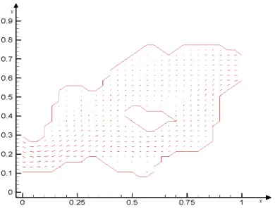
[image:7.612.316.523.75.270.2]

With the help of the described method, the results of numerical calculation with 30×30, 50×50 and 100×100 numbers of grid nodes were obtained. In Fig. 3, there are isolines of stream functions where vortex motion and flow around of obstacles are well observed. In Fig. 4, there are fields of the velocity vector and borders of vortex motion.

Figure 3: The Velocity Vector Field at The Grid 30×30

[image:7.612.99.294.219.369.2]

Figure 4: The Velocity Vector Field at the Grid 100×100

[image:7.612.315.524.311.488.2]

Figure 5: Isolines of the Stream Function at the Grid 50×50

Figure 6: Isolines of the Stream Function at the Grid 100×100

4. CONCLUSIONS

Modern requirements for authenticity of the received numerical results and reliability of program-methodical provision need a detailed testing and verification of the developed complex of programs. Testing of the developed methodology, algorithms and complex of programs was made based on tasks of progress in flow of viscous incompressible fluid [19].

This methodology of modeling incompressible fluid flow in the complex two dimensional geometrical domain deliver us from the small parameter and calculation of pressure for that there are not boundary conditions setting up the problem.

[image:7.612.107.285.390.564.2]

(8)

ACKNOWLEDGEMENT

The numerical methods of Navier-Stokes equation solution are studied in the work in the biconnected domain and executed within the State budget project. Number of State registration #0112РК02921, inventory number: 0214РК00220.

REFERENCES:

[1] P.N. Vabishchevich, Methods of fictitious domains in boundary value problems of mathematical physics. Moscow: Moscow State University; 1991.

[2] Sh.S. Smagulov, The method of fictitious domains for Navier-Stokes equations. Novosibirsk: Preprint of USSR Academy of Sciences, Siberian Department of Computer Centre; 1979.

[3] K. Fletcher, Computational methods in fluid dynamics. Vol. 1, 2. Moscow: Mir; 1991. [4] Zh. Baldybek, “The method of supplemented

domains for a nonlinear boundary value problem of the ocean”, Matematicheskiiy Zhurnal, Vol. 2, 2002, pp. 41–50.

[5] A.T. Mukhametzhanov, M.O. Otel’bayev, S.S. Smagulov, “On a method of fictitious domains for nonlinear boundary value problems”,

Vychislitelniye Tekhnologii, Vol. 3, No. 4, 1998, pp. 41–64.

[6] Sh.S. Smagulov, M.O. Otel’bayev, “On a new method of approximate solutions of nonlinear equations in an arbitrary domain”,

Vychislitelniye Tekhnologii, Vol. 6, No. 6, 2001, pp. 93–107.

[7] N.T. Danayev, “On one possibility of the numerical construction of orthogonal grids”,

Chislen. Metody Mekhan. Sploshnoy Sredy,

Vol. 14, 1983, pp. 42–53.

[8] Sh.S. Smagulov, N.T. Danayev, N.M. Temirbekov, “The numerical solution of the Navier-Stokes equations for the incompressible fluid in the channels with a porous rate”, Prikladnaya Mekhanika i

Tekhnicheskaya Fizika, Vol. 36, 1995, pp. 21–

29.

[9] N.N. Yanenko, N.T. Danayev, V.D. Liseikin, “On the variational method of grid generation”, Chislennyye Metody Mekhaniki Sploshnoy Sredy, Vol. 8, No. 4, 1977, pp. 157–163.

[10] A.A. Samarskiy, The theory of difference schemes. Moscow: Nauka; 1983.

[11] V.D. Liseikin, Yu.I. Shokin, I.A. Vaseva, Yu.V. Likhanova, The technology of construction of difference grids. Novosibirsk: Nauka; 2009.

[12] Yu.I. Shokin, N.T. Danayev, G.S. Khakimzyanov, N.Yu. Shokina, Lectures on the difference scheme on moving grids. In 3 parts: Part 2: Tasks for equations in partial differential coefficients with two space variables: Textbook. Almaty: Al-Farabi Kazakh National University; 2008.

[13] V.D. Liseikin, “Review of the design methods of structural adaptive grids”, Zhurnal

Vychislitel'nykh Matematiki i

Matematicheskoy Fiziki, Vol. 36, 1996, p. 39. [14] G.S. Khakimzyanov, V.D. Liseikin, A.S.

Lebedev, “Development of the design methods of adaptive grids”, Vychislitel'nyye Tekhnologii, Vol. 7, 2002, pp. 93–107. [15] N.M. Temirbekov, E.M. Mnafiyanov, E.A.

Malgazhdarov, A. Bailova, “Heat-mass transfer of incompressible fluid in biconnected domains with an arbitrary curvilinear boundary”, Mathematical Modeling of Scientific and Technological, Oil and Gas Producing Industry: Proceedings of the VI

International Kazakh-Russian

Scientific-Practical Conference, L. Gumilyov Eurasian

National University, Astana (Kazakhstan), October 11-12, 2007, pp. 317-322.

[16] J.F. Thompson, Z.U.A. Warsi, C.W. Mastin, Numerical grid generation, foundations and applications. New York, etc.: Elsevier; 1985. [17] V.P. Sirochenko, “Numerical modeling of

convective flows of the viscous fluid in multiconnected domains”, Proceedings of the

International Conference RDAMM-2001,

Vychislitelniye Tekhnologii, Novosibirsk (Russia), 2001, Vol. 6, No. 2, pp. 554–562. [18] A.A. Samarskiy, A.V. Gulin, Numerical

methods. Moscow: Nauka; 1989.