SVM BASED AUTOMATIC MEDICAL DECISION SUPPORT
SYSTEM FOR MEDICAL IMAGE
1JOSEPHINE SUTHA.V, 2Dr.P.LATHA
1Sardar Raja College Of Engineering, Tirunelveli, India 2Government College Of Engineering, Tirunelveli,India
E-mail: [email protected] [email protected]
ABSTRACT
An approach for automatic classification of Magnetic Resonance Image (MRI) is presented in this paper. In modern hospitals a vast amount of MR images are produced in the day to day life. So, an input image based automatic medical image retrieval system is now a necessity. In this paper, extracted features are classified using Support Vector Machine (SVM) with Radial Basis Function (RBF). The performance of SVM for varying parameters is investigated. Proposed system showed high classification accuracies (on an average > 99%) for all the datasets used in the experiments. Experimental results and performance comparisons with state-of-the-art techniques show that the proposed scheme is efficient in brain MR image classification.
Keywords: Magnetic Resonance Image, SIFT, Tumor, Support Vector Machine,
1. INTRODUCTION
Brain tumors are very common toxic disease .Also it is a complicated one to identify and to be treated. Diagnosis of brain tumor is one of the active research area .To improve the diagnosis of head MRI, special Medical Decision Support System have been extensively examined and implemented. But even in automated systems, there are various hitches. This turns the society to implement an automated brain tumor classification with increased accuracy and speed.
Magnetic Resonance Imaging is the study in which the structure and function of brain can be studied by doctors and researchers. To identify the Initial stage of the tumor is a tiresome process even for the experienced doctors. Society needs a very high quality classification system to speed up the process if the doctor finds as a tumor. If SIFT technique can be applied with the proper image dataset, it would be a simple thing for doctors to identify the location of the tumors. Also the treatment could be started in time and valued human lives would be saved. This work introduces an automated tumor recognition system [9] for MRI brain images.
In the last decades, many methods have been proposed to classify brain MR images. This
includes automatic classification of normal and abnormal images using SVM classifier developed by Daljit Singh [7] proposed a technique for Tumor Detection and Classification using Decision Tree. Wiselin [11] developed a method for abnormal MRI volume identification using Fuzzy C-Means algorithm. Selvaraj [4] built-up a technique for MRI Slices Classification Using Least Squares Support Vector Machine. The latest development in data classification has focused more on SVMs as it produces higher accuracy than other algorithms. The prime objective of the study is to implement an automatic MR image classification system with high accuracy rate.
2. SYSTEM DESCRIPTION:
this system a sample of 110 MR brain images were collected. 60 images are taken as normal brain and remaining 50 images are taken as abnormal brain. 60 images are used for training phase
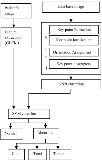
Figure 1: Stages For Detecting Tumor Using SIFT
and remaining 50 images are used for testing: out of which11 is normal and 48 are abnormal which are of bleed, clot, and tumor. MR Images with the same resolution and of T2 Weighted are considered for evaluation. Various image processing techniques have been applied in both training and testing phase. Precisely, techniques like pre-processing, feature extraction, KNN clustering, SIFT, classification and Diagnosis been used. The pre-processing and feature extraction technique are common for both training and test phase. Images are required to be preprocessed for feature extraction process.R2013b MATLAB version is used in the proposed work to get high accuracy of results.
2.1 Feature Extraction
Feature extraction has been done using GLCM. Gray Level Co-occurrence Matrix (GLCM) method is a way of extracting statistical texture features. In GLCM matrix Repeated pixels
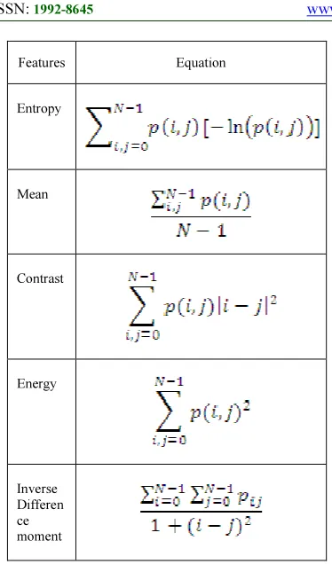
of an input image with a Certain intensity is considered as “i” .Other pixels with certain distance‘d’ is taken as “j”. From the above two parameters GLCM calculates the co-occurrence matrix. Thus the original data set will be reduced .The extracted features are Entropy, Mean, Contrast , Energy and Inverse Difference moment .These five statistic features have been used to distinguish between normal and abnormal image of a patient. By using following equations, different textural features have been calculated which can be used to train the SVM classifier.
2.2 SIFT (Scale Invariant Feature Transform):
SIFT has been proved to give accurate results and quick process as it is invariant to scale, orientation and minor affine changes. This transformation, transforms the image data into scale-invariant coordinates relative to its local features. Other techniques such as neuro-fuzzy logic and ANN based classifier could not be used more than couple of years as because of the age differentiation among the patient’s image and the data base images. But SIFT could be used up to 10 years [12] as it is scale invariant. This transform consists of four stages which are discussed below
2.2.1scale-space extrema detection:
This stage collects interested points, in the image which are called key points. Algorithm for Scale-space extrema detection is given below: 1. The input image is convolved with Gaussian filters at dissimilar scales.
2. The same output is grouped by octave.
3. Next difference of successive Gaussian blurred images is taken.
Identifying DoG images, key points are acknowledged for local minima/maxima of the DoG images across different scales. There is a need to find points that give information about the objects in the image. The information about the objects is around the object’s edges. Commonly image is represented in such a way that it gives edges along the extrema points.
Table1: Mathematical Statements Used To
Evaluate Various Features
Clot Bleed Tumor
Patient’s image
Feature extraction (GLCM)
SVM classifier
Data base image
Abnormal Normal
S
I
F
T
Key point Extraction
Key point localization
Orientation Assignment
Key pointdescriptors
2.2.2 key point localization:
In this stage filtering of Key points are done .Output of Scale-space extrema detection produces many more key points. All of them are not good, some of which are unstable. As a result a detailed fit is needed to the nearby data for the exact location, scale, and ratio of principal curvatures. This in turn allows some points to be rejected that have low contrast along an edge.
2.2.3 orientation assignment:
Orientation assignment corresponds to the representation which is invariant to rotation. For each sample point, gradient’s magnitude and orientation is calculated. An orientation histogram with 36 bins is created, with 10 degrees for each bin. Each sample in the neighboring window is added to a histogram bin. The histogram bin is weighted by its gradient magnitude and by a Gaussian-weighted circular window with 1.5 times that of the scale of the key point. The peaks in this histogram correspond to dominant orientation correspond to dominant orientations. When the histogram process is completed, the orientations corresponding to the highest peak and local peaks have to be calculated. If the orientations are within 80% of the highest peaks, then that orientations are assigned to the key point.
2.2.4 key point descriptor:
Key point descriptor is distinctive to Key point representation. Previous steps found key point locations at particular scales and assigned orientations to them. Key point descriptor is calculated using a region
around the key point as opposed to directly from the key point for robustness.
2.3 K Nearest Neighbour (k-NN) Clustering:
Matching of Key points were done by K-NN algorithm for classification purpose. The k-nearest neighbour algorithm is the simplest one among all the machine learning algorithms. At this juncture an object is classified by a bulk vote of its neighbours, by way of the object being assigned to the class. The most common amongst its k nearest neighbours (k is a positive integer, typically small). If k = 1, then the object is simply assigned to the class of its nearest neighbor.
2.4 Support Vector Machine (SVM):
[image:3.595.93.280.110.428.2]This classification algorithm is based on SVM classifier. SVM is binary classifier; it is used to classify the extracted features intotwo classes. In the proposed work it classifies as normal and abnormal images along with type of abnormality. In Brain MRI images; class 0 is defined for normal images and class 1 is defined for abnormal images.
Table 2: Classifier Recital Table
Method
SVM with SIFT(Proposed method)
SVM(Reference 1)
kernel
A
c
cu
ra
cy
S
pe
ci
fi
ci
ty
S
ens
it
ivi
ty
A
c
cu
ra
cy
S
pe
ci
fi
ci
ty
S
ens
it
ivi
ty
RBF 99 97.1 99.7 98 96.4 92
Linear 95 93.4 95.1 94 90.7 87.2
Quadratic 97 94.7 97.3 97 92.4 90.8
Table 3:Performance Table For Different Classifiers
Features Equation
Entropy
Mean
Contrast
Energy
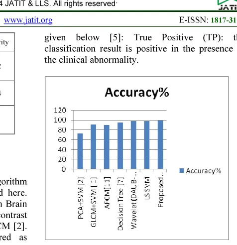
[image:3.595.305.489.507.684.2]3. EXPERIMENTAL RESULTS
SVM classification with SIFT algorithm for Brain MRI image have been proposed here. Proposed method is executed on real human Brain MR Images. For Normal Brain images contrast value varies from 0.7000 to 0.7550 for GLCM [2]. Images outside this range are considered as abnormal images. As GLCM gives utmost classification accuracy; images are further categorized into sort of existing abnormalities. If mean value lie 14.0000 to 14.5000 then patient is suffering from bleed. For clot the mean value lie 26.1500 to 27.8200 and for tumor mean value lie 24.6500 to 26.1200.
3.1 Performance Measures:
[image:4.595.262.500.95.341.2]Exactness of the proposed system could have been calculated by means of certain
Table 4: Accuracy For Various Classifiers
classification Technique Accuracy(%)
PCA+SVM [2] 73.07
GLCM+SVM [ 1] 90.83
AFCM[11] 90.10
Decision Tree [7] 96.00
Wavelet (DAUB-4) + PCA
+ SVM-RBF[ 3] 98.7
LS SVM 98.92
Proposed Method[4] 99.43
parameters known as True Positive, False Positive, True Negative And False Negative Which are
given below [5]: True Positive (TP): the classification result is positive in the presence of the clinical abnormality.
Figure 4: Accuracy Of Different Classifiers In Diagrammatic Representation
True Negative (TN): the classification result is negative in the absence of the clinical abnormality. False Positive (FP): the classification result is positive in the absence of the clinical abnormality. False Negative (FN): the classification result is negative in the presence of the clinical abnormality.
(1)
(2)
(3)
Classifier
Type Accuracy Specificity Sensitivity
Proposed
method 99.43 97.12 99.72
LS-SVM[4] 98.64 95.5 99.64
Neural
classifier[4] 92.37 85.39 94.6
[image:4.595.87.243.503.705.2]Figure 3: Performance Of Two Classifiers
As SIFT could be used up to 10 yearsof data base images, this can be taken as a limitation of the proposed work. This restriction can be clarified in future by another algorithm.
4. CONCLUSION:
This paper gives a boon to computerized decision system for the MR Image using SVM with SIFT. SIFT confirms to be the capable one as it is invariant to transformation, scale and rotation. Also, its implementation is quite simple and the expenditure is also very low. Faltering result shows that the technique is effective with greater accuracy. Proposed method is compact in implementation and effective in classification. Above said result will be of great reputation for brain tumor detection and classification. Hence this technique can be used for data supervision in hospitals and for tele-radiology.
REFERENCES:
[1]Rosy Kumari , “SVM Classification an Approach on Detecting Abnormality in Brain MRI Images”, International Journal of
Engineering Research and Application ,Vol. 3,
No. 4, 2013,pp.1686-1690.
[2] Daljit Singh, Kamaljeet Kaur , “Classification of Abnormalities in Brain MRI Images Using GLCM”, PCA and SVM ,International Journal
of Engineering and Advanced Technology ,
Vol.1, No.6, 2012,pp. 243-248.
[3] Mubashir Ahmad, Mahmood ul-Hassan, Imran Shafi, Abdelrahman Osman , “Classification of Tumors in Human Brain MRI using
Wavelet and Support Vector Machine”, IOSR
Journal of Computer Engineering, Vol. 8, No.
2, 2012, pp 25-31.
[4] H. Selvaraj, S. Thamarai Selvi, D. Selvathi, L. Gewali, “Brain MRI Slices Classification Using Least Squares Support Vector Machine”, IC-MED ,Vol. 1, No. 1, 2007, pp.21 -33.
[5] Carlos A. Parra, Khan Iftekharuddin ,Robert Kozma, “Automated Brain Data Segmentation and Pattern Recognition Using ANN”, Computational Intelligence, Robotics and
Autonomous Systems (CIRAS 03), 2003.
[6] Alan Wee-Chung Liew, Hong Yan, “Current Methods in the Automatic Tissue Segmentation of 3D Magnetic Resonance Brain Images”, Current Medical Imaging
Reviews, Vol.2, No.1, 2006,pp.1-13.
[7] Janki Naik , Sagar Patel , “Tumor Detection and Classification using Decision Tree in Brain MRI” , International Journal Of
Engineering Development And Research,
Vol.1.No.1, 2013,pp.49-53.
[8] Cuadra M, Pollo C, Bardera A, Cuisenaire O, Villemure JG, Thiran JP, “Atlas-based segmentation of pathological MR brain images using a model of lesion growth”, IEEE Trans
Med Imaging,Vol.23,No.10,2004,pp.1301–
1314.
[9] D. Jude Hemanth, C.Kezi Selva Vijila and J.Anitham , “Application of Neuro-Fuzzy Model for MR Brain Tumor Image Classification”, International Journal of Biomedical Soft Computing and Human
Sciences, Vol.16, No.1, 2010, pp. 95-102.
[10] L. Hall, A. Bensaid, L. Clarke, M. Silbiger, R. Velthuizen, and J. Bezdek, “A comparison of neural network and fuzzy clustering techniques in segmenting magnetic resonance images of the brain”, IEEE Trans. Neural
Networks, Vol. 3,1992, pp. 672–682.
[11] G. Wiselin Jiji, G. Evelin Suji , “MRI Brain Image Segmentation using Advanced Fuzzy C-Means Algorithm”, International Journal of
Computer Applications, Vol. 56,No.9, 2012,
pp.9-14.
[12] Arijita Pani, Priyanka Shende, Mrunmayi Dhumal, Kajal Sangle and Prof. Sankirti Shiravale, “Advantages Of Using SIFT For Brain Tumor Detection”, International Journal of Students Research in Technology &