SRC TN 1997 030A pdf

SRC Technical Note

1997 - 030a

December 9, 1997

Corrected December 25, 1997

Composition: A Way to Make Proofs Harder

Leslie Lamport

d i g i t a l

Systems Research Center

130 Lytton Avenue Palo Alto, California 94301

http://www.research.digital.com/SRC/

Composition: A Way to Make Proofs Harder

Leslie Lamport

Abstract

Contents

1 Introduction 2

2 The Mathematical Laws of Composition 2

3 Describing a System with Mathematics 3

3.1 Discrete Dynamic Systems . . . 4

3.2 An Hour Clock . . . 4

3.2.1 A First Attempt . . . 4

3.2.2 Stuttering . . . 5

3.2.3 Fairness . . . 6

3.3 An Hour-Minute Clock . . . 7

3.3.1 The Internal Specification . . . 7

3.3.2 Existential Quantification . . . 8

3.4 Implementation and Implication . . . 9

3.5 Invariance and Step Simulation . . . 11

3.6 A Formula by any Other Name . . . 11

4 Invariance in a Pseudo-Programming Language 11 4.1 The Owicki-Gries Method . . . 12

4.2 Why Bother? . . . 14

5 Refinement 15 5.1 Refinement in General . . . 15

5.2 Hierarchical Refinement . . . 16

5.3 Interface Refinement . . . 16

6 Decomposing Specifications 17 6.1 Decomposing a Clock into its Hour and Minute Displays . . . 17

6.2 Decomposing Proofs . . . 19

6.3 Why Bother? . . . 21

6.4 When a Decomposition Theorem is Worth the Bother . . . 23

7 Composing Specifications 23

8 Conclusion 24

1

Introduction

When an engineer designs a bridge, she makes a mathematical model of it and reasons mathematically about her model. She might talk about calculating rather than reasoning, but calculating√2 to three decimal places is just a way of proving

|√2−1.414|<10−3. The engineer reasons compositionally, using laws of math-ematics to decompose her calculations into small steps. She would probably be mystified by the concept of compositional reasoning about bridges, finding it hard to imagine any form of reasoning that was not compositional.

Because computer systems can be built with software rather than girders and rivets, many computer scientists believe these systems should not be modeled with the ordinary mathematics used by engineers and scientists, but with something that looks vaguely like a programming language. We call such a language a

pseudo-programming languages (PPL). Some PPLs, such as CSP, use constructs of

ordi-nary programming languages. Others, like CCS, use more abstract notation. But, they have two defining properties: they are specially designed to model computer systems, and they are not meant to implement useful, real-world programs.

When using a pseudo-programming language, compositional reasoning means writing a model as the composition of smaller pseudo-programs, and reasoning separately about those smaller pseudo-programs. If one believes in using PPLs to model computer systems, then it is natural to believe that decomposition should be done in terms of the PPL, so compositionality must be a Good Thing.

We adopt the radical approach of modeling computer systems the way engi-neers model bridges—using mathematics. Compositionality is then a trivial con-sequence of the compositionality of ordinary mathematics. We will see that the compositional approaches based on pseudo-programming languages are analogous to performing calculations about a bridge design by decomposing it into smaller bridge designs. While this technique may occasionally be useful, it is hardly a good general approach to bridge design.

2

The Mathematical Laws of Composition

We will use the notation introduced in [10] to write hierarchical proofs. Two fundamental laws of mathematics are used to decompose proofs:

∧-Composition A⇒B

A⇒C

A⇒B∧C

∨-Composition A⇒C

B⇒C

A∨B ⇒C

Logicians have other names for these laws, but our subject is compositionality, so we adopt these names. A special case of∨-composition is:

Case-Analysis A∧B ⇒C

A∧ ¬B⇒C

A⇒C

The propositional∧- and∨-composition rules have the following predicate-logic generalizations:

∀-Composition (i ∈S)∧P ⇒Q(i)

P ⇒(∀i ∈S : Q(i))

∃-Composition (i ∈S)∧P(i)⇒Q

(∃i∈S : P(i))⇒Q Another rule that is often used (under a very different name) is

Act-Stupid A⇒C

A∧B ⇒C

We call it the act-stupid rule because it proves thatA∧B impliesC by ignoring the hypothesisB. This rule is useful whenB can’t help in the proof, so we need only the hypothesisA. Applying it in a general method, when we don’t know what

AandBare, is usually a bad idea.

3

Describing a System with Mathematics

3.1

Discrete Dynamic Systems

Our clock is a dynamic system, meaning that it evolves over time. The classic way to model a dynamic system is by describing its state as a continuous function of time. Such a function would describe the continuum of states the display passes through when changing from 12:49 to 12:50. However, we view the clock as a discrete system. Discrete systems are, by definition, ones we consider to exhibit discrete state changes. Viewing the clock as a discrete system means ignoring the continuum of real states and pretending that it changes from 12:49 to 12:50 with-out passing through any intermediate state. We model the execution of a discrete system as a sequence of states. We call such a sequence a behavior. To describe a system, we describe all the behaviors that it can exhibit.

3.2

An Hour Clock

3.2.1 A First Attempt

To illustrate how systems are described mathematically, we start with an even sim-pler example than the hour-minute clock—namely, a clock that displays only the hour. We describe its state by the value of the variablehr. A typical behavior of this system is

[hr =11] → [hr =12] → [hr =1] → [hr =2] → · · ·

We describe all possible behaviors by an initial predicate that specifies the possible initial values ofhr, and a next-state relation that specifies how the value ofhr can change in any step (pair of successive states).

The initial predicate is justhr ∈ {1, . . . ,12}. The next-state relation is the following formula, in which hr denotes the old value and hr

0 _{denotes the new}

value.

((hr =12) ∧ (hr

0 _{=1)) ∨ ((}

hr 6=12) ∧ (hr

0₌

hr+1))

This kind of formula is easier to read when written with lists of conjuncts or dis-juncts, using indentation to eliminate parentheses:

∨ ∧hr =12

∧hr

0 ₌₁

∨ ∧hr 6=12

∧hr

0 ₌

hr +1

There are many ways to write the same formula. Borrowing some notation from programming languages, we can write this next-state relation as

hr

0 _{= if}

This kind of formula, a Boolean-valued expression containing primed and un-primed variables, is called an action.

Our model is easier to manipulate mathematically if it is written as a single formula. We can write it as

∧

hr

∈ {1, . . . ,12}

∧2(

hr

0 _=if

hr

_{=12 then 1 else}

hr

₊₁₎ (1)

This is a temporal formula, meaning that it is true or false of a behavior. A state predicate like

hr

∈ {1, . . . ,12}is true for a behavior iff it is true in the first state. A formula of the form2

N

asserts that the action

N

holds on all steps of the behavior. By introducing the operator2, we have left the realm of everyday mathematics and entered the world of temporal logic. Temporal logic is more complicated than ordinary mathematics. Having a single formula as our mathematical description is worth the extra complication. However, we should use temporal reasoning as little as possible. In any event, temporal logic formulas are still much easier to reason about than programs in a pseudo-programming language.

3.2.2 Stuttering

Before adopting (1) as our mathematical description of the hour clock, we ask the question, what is a state? For a simple clock, the obvious answer is that a state is an assignment of values to the variable

hr

. What about a railroad station with a clock? To model a railroad station, we would use a number of additional variables, perhaps including a variable

sig

to record the state of a particular signal in the station. One possible behavior of the system might be

  

hr =11

sig =“red”

...

   →   

hr =12

sig =“red”

...

   →   

hr =12

sig =“green”

...

   →   

hr =12

sig =“red”

...

   →   

hr =1

sig =“red”

...

 

 → · · ·

We would expect our description of a clock to describe the clock in the railroad station. However, formula (1) doesn’t do this. It asserts that

hr

is incremented in every step, but the behavior of the railroad station with clock includes steps like the second and third, which change

sig

but leave

hr

unchanged.

x

+

y

=1, doesn’t assert that there is no

z

. It simply says nothing about the value of

z

. In other words, the formula

x

+

y

=1 is not an assertion about some universe containing only

x

and

y

. It is an assertion about a universe containing

x

,

y

, and all other variables; it constrains the values of only the variables

x

and

y

.

Similarly, a mathematical formula that describes a clock should be an assertion not about the variable

hr

, but about the entire universe of possible variables. It should constrain the value only of

hr

and should allow arbitrary changes to the other variables—including changes that occur while the value of

hr

stays the same. We obtain such a formula by modifying (1) to allow “stuttering” steps that leave

hr

unchanged, obtaining:

∧

hr

∈ {1, . . . ,12}

∧2

∨hr0 =if hr =12 then 1 else hr+1

∨hr0 =hr

(2)

Clearly, every next-state relation we write is going to have a disjunct that leaves variables unchanged. So, it’s convenient to introduce the notation that [

A

]v equals

A

∨(

v

0 ₌

v

_{), where}

v

0_{is obtained from the expression}

v

_{by priming all its free}

variables. We can then write (2) more compactly as

∧

hr

∈ {1, . . . ,12}

∧2[

hr

0=if

hr

=12 then 1 else

hr

+1]hr

(3)

This formula allows behaviors that stutter forever, such as

[

hr

=11] → [

hr

=12] → [

hr

=12] → [

hr

=12] → · · ·

Such a behavior describes a stopped clock. It illustrates that we can assume all behaviors are infinite, because systems that halt are described by behaviors that end with infinite stuttering. But, we usually want our clocks not to stop.

3.2.3 Fairness

To describe a clock that doesn’t stop, we must add a conjunct to (3) to rule out infinite stuttering. Experience has shown that the best way to write this conjunct is with fairness formulas. There are two types of fairness, weak and strong, expressed with the WF and SF operators that are defined as follows.

WFv(

A

) If

A

∧(

v

0 6=

v

)is enabled forever, then infinitely many

A

∧(

v

0 6=

v

) steps must occur.

SF_v(

A

) If

A

∧(

v

06=

v

)is enabled infinitely often, then infinitely many

A

∧(

v

06=

The

v

0 6=

v

conjuncts make it impossible to use WF or SF to write a formula that rules out finite stuttering.

We can now write our description of the hour clock as the formula5, defined by

N

1

=

hr

0_=if

hr

_{=12 then 1 else}

hr

₊₁

5 =1 (

hr

∈ {1, . . . ,12})∧ 2[

N

]hr ∧ WFhr(

N

)

The first two conjuncts of5(which equal (3)), express a safety property. Intu-itively, a safety property is characterized by any of the following equivalent condi-tions.

• It asserts that the system never does something bad.

• It asserts that the system starts in a good state and never takes a wrong step.

• It is finitely refutable—if it is violated, then it is violated at some particular point in the behavior.

The last conjunct of 5(the WF formula) is an example of a liveness property. Intuitively, a liveness property is characterized by any of the following equivalent conditions.

• It asserts that the system eventually does something good.

• It asserts that the system eventually takes a good step.

• It is not finitely refutable—it is possible to satisfy it after any finite portion of the behavior.

Formal definitions of safety and liveness are due to Alpern and Schneider [4]. Safety properties are proved using only ordinary mathematics (plus a couple of lines of temporal reasoning). Liveness properties are proved by combining tem-poral logic with ordinary mathematics. Here, we will mostly ignore liveness and concentrate on safety properties.

3.3

An Hour-Minute Clock

3.3.1 The Internal Specification

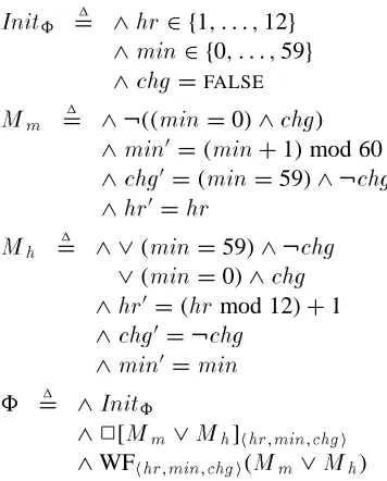
Init

8 = ∧1

hr

∈ {1, . . . ,12}

∧

min

∈ {0, . . . ,59}

∧

chg

=FALSE

M

m = ∧ ¬((1

min

=0)∧

chg

)

∧

min

0 ₌₍

min

_{+1)mod 60}

∧

chg

0 ₌₍

min

_{=59)∧ ¬}

chg

∧

hr

0 ₌

hr

M

h = ∧ ∨1 (

min

=59)∧ ¬

chg

∨(

min

=0)∧

chg

∧

hr

0 ₌₍

hr

_{mod 12)+1}

∧

chg

0 _{= ¬}

chg

∧

min

0 ₌

min

8 _{= ∧}1

Init

8

∧2[

M

m ∨

M

h]hhr,min,chgi

[image:11.612.215.393.141.362.2]

∧WF_hhr_,min_,chg_i(

M

m ∨

M

h)

Figure 1: The internal specification of an hour-minute clock.

actual times at which state changes occur, these transient states are no different from the states when the clock displays the “correct” time.

Figure 1 defines a formula8that describes the hour-minute clock. It uses an additional variable

chg

that equalsTRUE when the display is in a transient state. Action

M

m describes the changing of

min

; action

M

h describes the changing of

hr

. The testing and setting of

chg

by these actions is a bit tricky, but a little thought reveals what’s going on. Action

M

h introduces a gratuitous bit of cleverness to re-move the if/then construct from the specification of the new value of

hr

. The next-state relation for the hour-minute clock is

M

m ∨

M

h, because a step of the clock increments either

min

or

hr

. Since h

hr

,

min chg

i0 equals h

hr

0,

min

0,

chg

0i, it equalsh

hr

,

min

,

chg

iiff

hr

,

min

, and,

chg

are all unchanged.

3.3.2 Existential Quantification

Formula8 of Figure 1 contains the free variables

hr

,

min

, and

chg

. However, the description of a clock should mention only

hr

and

min

, not

chg

. We need to “hide”

chg

. In mathematics, hiding means existential quantification. The formula

clock is∃∃∃∃∃∃

chg

:8. The quantifier∃∃∃∃∃∃ is a temporal operator, asserting that there is a sequence of values of

chg

that makes8true. The precise definition of∃∃∃∃∃∃ is a bit subtle and can be found in [9].

3.4

Implementation and Implication

An hour-minute clock implements an hour clock. (If we ask someone to build a device that displays the hour, we can’t complain if the device also displays the minute.) Every behavior that satisfies the description of an hour-minute clock also satisfies the description of an hour clock. Formally, this means that the formula

(∃∃∃∃∃∃

chg

:8)⇒5is true. In mathematics, if something is true, we should be able to prove it. The rules of mathematics allow us to decompose the proof hierarchically. Here is the statement of the theorem, and the first two levels of its proof. (See [10] for an explanation of the proof style.)

Theorem 1 (∃∃∃∃∃∃

chg

: 8)⇒5

h1i1. 8⇒5

h2i1.

Init

₈⇒

hr

∈ {1, . . . ,12}

h2i2. 2[

M

m ∨

M

h]hhr,min,chgi ⇒2[

N

]hr

h2i3. 8⇒WFhr(

N

)

h2i4. Q.E.D.

PROOF: Byh2i1–h2i3 and the∧-composition and act-stupid rules.

h1i2. Q.E.D.

PROOF: By h1i1, the definition of8, and predicate logic1, since

chg

does not occur free in5.

Let’s now go deeper into the hierarchical proof. The proof ofh2i1 is trivial, since

Init

8 contains the conjunct

hr

∈ {1, . . . ,12}. Proving liveness requires more

temporal logic than we want to delve into here, so we will not show the proof of

h2i3 or of any other liveness properties. We expand the proof ofh2i2 two more levels as follows.

h2i2. 2[

M

m ∨

M

h]hhr,min,chgi ⇒2[

N

]hr

h3i1. [

M

m∨

M

h]_hhr_,min_,chg_i ⇒[

N

]hr

h4i1.

M

m ⇒[

N

]hr

h4i2.

M

h ⇒[

N

]hr

h4i3. (h

hr

,

min

,

chg

i0= h

hr

,

min

,

chg

i)⇒[

N

]hr

h4i4. Q.E.D.

PROOF: Byh4i1–h4i3 and the∨-composition rule.

1_{We are actually reasoning about the temporal operator∃∃∃∃∃∃ rather than ordinary existential}

h3i2. Q.E.D.

PROOF: Byh3i1 and the rule

A

⇒

B

2

A

⇒2

B

.

The proof of h4i1 is easy, since

M

m implies

hr

0 =

hr

. The proof of h4i3 is equally easy. The proof ofh4i2 looks easy enough.

h4i2.

M

h ⇒[

N

]hr

PROOF:

M

h ⇒

hr

0 = (

hr

mod 12)+1

⇒

hr

0 _{= if}

hr

_{=12 then 1 else}

hr

₊₁

1

=

N

However, this proof is wrong! The second implication is not valid. For example, if

hr

equals 25, then the first equation asserts

hr

0 = 2, while the second asserts

hr

0 _{= 26. The implication is valid only under the additional assumption}

hr

_∈

{1, . . . ,12}.

Define

Inv

to equal the predicate

hr

∈ {1, . . . ,12}. We must show that

Inv

is true throughout the execution, and use that fact in the proof of steph4i2. Here are the top levels of the corrected proof.

h1i1. 8⇒5

h2i1.

Init

₈⇒

hr

∈ {1, . . . ,12}

h2i2.

Init

₈∧2[

M

m ∨

M

h]hhr,min,chgi⇒2

Inv

h2i3. 2

Inv

∧2[

M

m ∨

M

h]hhr,min,chgi ⇒2[

N

]hr

h2i4. 2

Inv

∧8⇒WFhr(

N

)

h2i5. Q.E.D.

PROOF: Byh2i1–h2i4, and the∧-composition and act-stupid rules.

h1i2. Q.E.D.

PROOF: By h1i1, the definition of 8, and predicate logic, since

chg

does not occur free in5.

The high-level proofs ofh2i2 andh2i3 are

h2i2.

Init

₈∧2[

M

m ∨

M

h]hhr,min,chgi⇒2

Inv

h3i1.

Init

₈⇒

Inv

h3i2.

Inv

∧[

M

m ∨

M

h]_hhr_,min_,chg_i⇒

Inv

0

h3i3. Q.E.D.

PROOF: Byh3i1,h3i2 and the rule

P

∧[

A

]v ⇒

P

0

P

∧2[

A

]v ⇒2

P

.

h2i3. 2

Inv

∧2[

M

m ∨

M

h]hhr,min,chgi ⇒2[

N

]hr

h3i1.

Inv

∧[

M

m ∨

M

h]_hhr_,min_,chg_i⇒[

N

]hr

h3i2. Q.E.D.

PROOF: Byh3i1 and the rules

A

⇒

B

2

A

⇒2

B

The further expansion of the proofs is straightforward and is left as an exercise for the diligent reader.

3.5

Invariance and Step Simulation

The part of the proof shown above is completely standard. It contains all the temporal-logic reasoning used in proving safety properties. The formula

Inv

satis-fyingh2i2 is called an invariant. Substeph3i2 of steph2i3 is called proving step

simulation. The invariant is crucial in this step and in steph2i4 (the proof of live-ness). In general, the hard parts of the proof are discovering the invariant, substep

h3i2 of steph2i2 (the crucial step in the proof of invariance), step simulation, and liveness.

In our example,

Inv

asserts that the value of

hr

always lies in the correct set. Computer scientists call this assertion type correctness, and call the set of correct values the type of

hr

. Hence,

Inv

is called a type-correctness invariant. This is the simplest form of invariant. Computer scientists usually add a type system just to handle this particular kind of invariant, since they tend to prefer formalisms that are more complicated and less powerful than simple mathematics.

Most invariants express more interesting properties than just type correctness. The invariant captures the essence of what makes an implementation correct. Find-ing the right invariant, and provFind-ing its invariance, suffices to prove the desired safety properties of many concurrent algorithms. This is the basis of the first practi-cal method for reasoning about concurrent algorithms, which is due to Ashcroft [5].

3.6

A Formula by any Other Name

We have been calling formulas like8and5“descriptions” or “models” of a sys-tem. It is customary to call them specifications. This term is sometimes reserved for high-level description of systems, with low-level descriptions being called

imple-mentations. We make no distinction between specifications and impleimple-mentations.

They are all descriptions of a system at various levels of detail. We use the terms algorithm, description, model, and specification as different names for the same thing: a mathematical formula.

4

Invariance in a Pseudo-Programming Language

S

(i)

0

S

(i)_n

−1

{

A

(i)_n−1}

?

?

...

?

{

A

(i)

[image:15.612.265.343.126.278.2]

0}

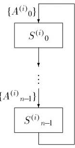
Figure 2: An Owicki-Gries style annotation of a process.

4.1

The Owicki-Gries Method

In the Owicki-Gries method [8, 11], the invariant is written as a program annota-tion. For simplicity, let’s assume a multiprocess program in which each process

i

in a set P of processes repeatedly executes a sequence of atomic instructions

S

(i)0, . . . ,

S

(i)_n−1. The invariant is written as an annotation, in which each statement

S

(i)_{j is preceded by an assertion}

A

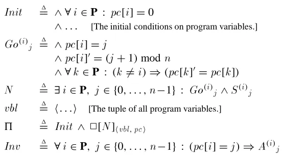
(i)_{j, as shown in Figure 2.}

To make sense of this picture, we must translate it into mathematics. We first rewrite each operation

S

(i)j as an action, which we also call

S

(i)j. This rewriting is easy. For example, an assignment statement

x

:=

x

+1 is written as the action

(

x

0 ₌

x

_{+1)∧(h. . .i}0 _{= h. . .i), where “. . . ” is the list of other variables. We}

represent the program’s control state with a variable

pc

, where

pc

[

i

] =

j

means that control in process

i

is immediately before statement

S

(i)j. The program and its invariant are then described by the formulas5and

Inv

of Figure 3.

We can derive the Owicki-Gries rules for proving invariance by applying the proof rules we used before. The top-level proof is:

Theorem 2 (Owicki-Gries) 5⇒2

I

h1i1.

Init

⇒

Inv

h1i2.

Inv

∧[

N

]_hvbl_,pc_i ⇒

Inv

0

h2i1.

Inv

∧

N

⇒

Inv

0

h2i2.

Inv

∧(h

vbl

,

pc

i0= h

vbl

,

pc

i)⇒

Inv

0

h2i3. Q.E.D.

PROOF: Byh2i1,h2i2, and the∨-composition rule.

Init

_{= ∧ ∀}1

i

_∈

P :

pc

[

i

]=0

∧. . . [The initial conditions on program variables.]

Go

(i)_{j = ∧}1

pc

[

i

]=

j

∧

pc

[

i

]0=(

j

+1)mod

n

∧ ∀

k

∈P : (

k

6=

i

)⇒(

pc

[

k

]0 =

pc

[

k

])

N

_{= ∃}1

i

_∈

P,

j

∈ {0, . . . ,

n

−1} :

Go

(i)j ∧

S

(i)j

vbl

_{= h. . .i}1

[The tuple of all program variables.]

5 ₌1

Init

_∧

2[

N

]hvbl,pci

Inv

_{= ∀}1

i

_∈

[image:16.612.166.444.139.293.2]

P,

j

∈ {0, . . . ,

n

−1} : (

pc

[

i

]=

j

)⇒

A

(i)j

Figure 3: The formulas describing the program and annotation of Figure 2.

PROOF: Byh1i1,h1i2, and the rule

P

∧[

A

]v ⇒

P

0

P

∧2[

A

]v ⇒2

P

.

The hard part is the proof of h2i1. We first decompose it using the ∀- and ∃ -composition rules.

h2i1.

Inv

∧

N

⇒

Inv

0

h3i1. 

∧∧

i

j

∈∈ {P0, . . . ,

n

−1}

∧

Inv

∧

Go

(i)_{j ∧}

S

(i)_j



 _⇒

_Inv

0

h4i1.       

∧

i

∈P

∧

j

∈ {0, . . . ,

n

−1}

∧

k

∈P

∧

l

∈ {0, . . . ,

n

−1}

∧

Inv

∧

Go

(i)_{j ∧}

S

(i)_j

      ⇒((

pc[k]0 =l)⇒(A(k)l)0)

h4i2. Q.E.D.

PROOF: Byh4i1, the definition of

Inv

, and the∀-composition rule.

h3i2. Q.E.D.

PROOF: Byh3i1, the definition of

N

, and the∃-composition rule.

h4i1.    

∧

i

,

k

∈P

∧

j

,

l

∈ {0, . . . ,

n

−1}

∧

pc

[

k

]0 =

l

∧

Inv

∧

Go

(i)_{j ∧}

S

(i)_j

  

 ⇒ (

A

(k)l)0

h5i1. CASE:

i

=

k

h6i1. 

∧_∧

i

_j

∈_{∈ {}P0, . . . ,

n

−1}

∧

A

(i)_{j ∧}

S

(i)_j



 _{⇒ (}

_A

(i)_j⊕1)0

h6i2. Q.E.D.

PROOF: By h6i1, the level-h5iassumption, the definition of

Inv

, and the act-stupid rule, since(

pc

[

i

]0=

l

)∧

Go

(i)j implies(

l

=

j

⊕1).

h5i2. CASE:

i

6=

k

h6i1. 

_∧∧

i

j

,_,

k

l

_{∈ {}∈P0, . . . ,

n

−1}

∧

A

(i)_{j ∧}

A

(k)_{l ∧}

S

(i)_j



 _{⇒ (}

A

(k)_l)0

h6i2. Q.E.D.

PROOF: By h6i1, the level-h5iassumption, the definition of

Inv

, and the act-stupid rule, since(

pc

[

k

]0 =

l

)∧

Go

(i)j implies(

pc

[

k

]=

l

), for

k

6=

i

, and(

pc

[

k

]=

l

)∧

Inv

implies

A

(k)l.

We are finally left with the two subgoals numberedh6i1. Summarizing, we see that to prove

Init

⇒2

Inv

, it suffices to prove the two conditions

A

(i)_{j ∧}

S

(i)_{j ⇒ (}

A

(i)_j⊕1)0

A

(i)_{j ∧}

A

(k)_{l ∧}

S

(i)_{j ⇒ (}

A

(k)_l)0

for all

i

,

k

in P with

i

6=

k

, and all

j

,

l

in{0, . . . ,

n

−1}. These conditions are called Sequential Correctness and Interference Freedom, respectively.

4.2

Why Bother?

We now consider just what have has been accomplished by describing by prov-ing invariance in terms of a pseudo-programmprov-ing language instead of directly in mathematics.

The difficulty of deciding what can and cannot be changed by an assignment state-ment is one of the things that makes the semantics of programming languages (both real and pseudo) complicated. By using mathematics, we avoid this problem com-pletely.

A major achievement of the Owicki-Gries method is eliminating the explicit mention of the variable

pc

. By writing the invariant as an annotation, one can write

A

(i)_{j instead of(}

pc

_[

i

_]=

j

_)⇒

A

(i)_{j. At the time, computer scientists seemed to}

think that mentioning

pc

was a sin. However, when reasoning about a concurrent algorithm, we must refer to the control state in the invariant. Owicki and Gries therefore had to introduce dummy variables to serve as euphemisms for

pc

. When using mathematics, any valid formula of the form

Init

∧2[

N

]v ⇒2

P

, for a state predicate

P

, can be proved without adding dummy variables.

One major drawback of the Owicki-Gries method arises from the use of the act-stupid rule in the proofs of the two steps numberedh6i2. The rule was applied without regard for whether the hypotheses being ignored are useful. This means that there are annotations for which steph2i1 (which asserts

N

∧

Inv

⇒

Inv

0) is valid but cannot be proved with the Owicki-Gries method. Such invariants must be rewritten as different, more complicated annotations.

Perhaps the thing about the Owicki-Gries method is that it obscures the un-derlying concept of invariance. We refer the reader to [6] for an example of how complicated this simple concept becomes when expressed in terms of a pseudo-programming language. In 1976, the Owicki-Gries method seemed like a major advance over Ashcroft’s simple notion of invariance. We have since learned better.

5

Refinement

5.1

Refinement in General

We showed above that an hour-minute clock implements an hour clock by proving

(∃∃∃∃∃∃

chg

: 8)⇒5. That proof does not illustrate the general case of proving that one specification implements another because the higher-level specification5has no internal (bound) variable. The general case is covered by the following proof outline, where

x

,

y

, and

z

denote arbitrary tuples of variables, and the internal variables

y

and

z

of the two specifications are distinct from the free variables

x

. The proof involves finding a function

f

, which is called a refinement mapping [1].

Theorem 3 (Refinement) (∃∃∃∃∃∃

y

: 8(

x

,

y

)) ⇒ (∃∃∃∃∃∃

z

: 5(

x

,

z

))

LET:

z

=1

f

(

x

,

y

)

h1i2. 8(

x

,

y

) ⇒ (∃∃∃∃∃∃

z

: 5(

x

,

z

))

PROOF: By h1i1 and predicate logic, since the variables of

z

are distinct from those of

x

.

The proof of steph1i1 has the same structure as in our clock example.

5.2

Hierarchical Refinement

In mathematics, it is common to prove a theorem of the form

P

⇒

Q

by in-troducing a new formula

R

and proving

P

⇒

R

and

R

⇒

Q

. We can prove that a lower-level specification∃∃∃∃∃∃

y

: 8(

x

,

y

) implies a higher-level specification

∃∃∃∃∃∃

z

:5(

x

,

z

)by introducing an intermediate-level specification∃∃∃∃∃∃

w

:9(

x

,

w

)and using the following proof outline.

LET: 9(

x

,

w

) =1 . . .

h1i1. (∃∃∃∃∃∃

y

: 8(

x

,

y

)) ⇒ (∃∃∃∃∃∃

w

: 9(

x

,

w

)) LET:

w

=1

g

(

x

,

y

)

. . .

h1i2. (∃∃∃∃∃∃

w

: 9(

x

,

w

)) ⇒ (∃∃∃∃∃∃

z

: 5(

x

,

z

)) LET:

z

=1

h

(

x

,

w

)

. . .

h1i3. Q.E.D.

PROOF: Byh1i1 andh1i2.

This proof method is called hierarchical decomposition. It’s a good way to explain a proof. By using a sequence multiple intermediate specifications, each differing from the next in only one aspect, we can decompose the proof into conceptually simple steps.

Although it is a useful pedagogical tool, hierarchical decomposition does not simplify the total proof. In fact, it usually adds extra work. Hierarchical decom-position adds the task of writing the extra intermediate-level specification. It also restricts how the proof is decomposed. The single refinement mapping

f

in the outline of the direct proof can be defined in terms of the two mappings

g

and

h

of the hierarchical proof by

f

(

x

,

y

)=1

h

(

x

,

g

(

x

,

y

)). The steps of a hierarchical proof can then be reshuffled to form a particular way of decomposing the lower levels of the direct proof. However, there could be better ways to decompose those levels.

5.3

Interface Refinement

net

, then the low-level specification must also describe the sending of messages on

net

.

We often implement a specification by refining the interface. For example, we might implement a specification6(

net

)of sending messages on

net

by a specifi-cation3(

tran

)of sending packets on a “transport layer” whose state is represented by a variable

tran

. A single message could be broken into multiple packets. Cor-rectness of the implementation cannot mean validity of3(

tran

)⇒6(

net

), since

3(

tran

)and6(

net

)have different free variables.

To define what it means for3(

tran

)to implement6(

net

), we must first define what it means for sending a set of packets to represent the sending of a message. This definition is written as a temporal formula

R

(

net

,

trans

), which is true of a behavior iff the sequence of values of

trans

represents the sending of packets that correspond to the sending of messages represented by the sequence of values of

net

. We call

R

an interface refinement. For

R

to be a sensible interface refine-ment, the formula3(

trans

)⇒ ∃∃∃∃∃∃

net

:

R

(

net

,

trans

)must be valid, meaning that every set of packet transmissions allowed by3(

trans

)represents some set of mes-sage transmissions. We say that3(

tran

)implements6(

net

)under the interface refinement

R

(

net

,

trans

)iff3(

tran

)∧

R

(

net

,

trans

)implies6(

net

).

6

Decomposing Specifications

Pseudo-programming languages usually have some parallel composition operator

k, where

S

1k

S

2 is the parallel composition of specifications

S

1 and

S

2. We ob-served in our hour-clock example that a mathematical specification

S

1 does not describe only a particular system; rather, it describes a universe containing (the variables that represent) the system. Composing two systems means ensuring that the universe satisfies both of their specifications. Hence, when the specifications

S

1and

S

2are mathematical formulas, their composition is just

S

1∧

S

2.

6.1

Decomposing a Clock into its Hour and Minute Displays

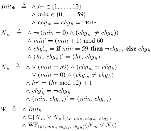
We illustrate how composition becomes conjunction by specifying the hour-minute clock as the conjunction of the specifications of an hour process and a minute process. It is simpler to do this if each variable is modified by only one process. So, we rewrite the specification of the hour-minute clock by replacing the variable

chg

with the expression

chg

h 6=

chg

m, where

chg

h and

chg

m are two new variables,

Init

9 = ∧1

hr

∈ {1, . . . ,12}

∧

min

∈ {0, . . . ,59}

∧

chg

_m =

chg

_h =TRUE

N

m = ∧ ¬((1

min

=0)∧(

chg

m 6=

chg

h))

∧

min

0₌₍

min

_{+1)mod 60}

∧

chg

0_{m =if}

min

_{=59 then¬}

chg

_{m else}

chg

_h

∧ h

hr

,

chg

_hi0 _{= h}

hr

_,

chg

_hi

N

h = ∧ ∨1 (

min

=59)∧(

chg

m =

chg

h)

∨(

min

=0)∧(

chg

m 6=

chg

h)

∧

hr

0₌₍

hr

_{mod 12)+1}

∧

chg

0

h = ¬

chg

h

∧ h

min

,

chg

_mi0_{= h}

min

_,

chg

_mi

9 _{= ∧}1

Init

9

∧2[

N

m ∨

N

h]hhr,min,chgm,chghi

[image:21.612.176.433.140.364.2]

∧WF_hhr_,min_,chg_m,chg_hi(

N

m ∨

N

h)

Figure 4: Another internal specification of the hour-minute clock.

is left as a nice exercise for the reader. The proof that∃∃∃∃∃∃

chg

h,

chg

m : 9 implies

∃∃∃∃∃∃

chg

: 8uses the refinement mapping

chg

=1 (

chg

h 6=

chg

m). The proof of the

converse implication uses the refinement mapping

chg

h =1

chg

∧(

min

=59)

chg

_m =1

chg

∧(

min

=0)

The specifications9h and9m of the hour and minute processes appear in Figure 5. We now sketch the proof that9is the composition of those two specifications.

Theorem 4 9 ≡ 9m ∧9h

Init

m = ∧1

min

∈ {0, . . . ,59}

∧

chg

_m =TRUE

Init

h = ∧1

hr

∈ {1, . . . ,12}

∧

chg

_h =TRUE

9_{h =}1

Init

h ∧2[

N

h]hhr,chghi ∧WFhhr,chghi(

N

h)

9_{m =}1

Init

h1i1.

Init

₉ ≡

Init

m ∧

Init

h

h1i2. 2[

N

m ∨

N

h]hhr,min,chgm,chghi ≡ 2[

N

m]hmin,chgmi ∧ 2[

N

h]hhr,chghi

h2i1. [

N

m ∨

N

h]_hhr_,min_,chg_m,chg_hi ≡ [

N

m]_hmin_,chg_mi ∧ [

N

h]_hhr_,chg_hi

h2i2. Q.E.D.

PROOF: Byh2i1 and the rules

A

⇒

B

2

A

⇒2

B

and 2(

A

∧

B

)≡2

A

∧2

B

.

h1i3. ∧9 ⇒ WF_hmin_,chg_mi(

N

m)∧WF_hhr_,chg_hi(

N

h)

∧9_m ∧9_h ⇒ WF_hhr_,min_,chg_m,chg_hi(

N

m ∨

N

h)

h1i4. Q.E.D.

PROOF: Byh1i1–h1i3.

Ignoring liveness (steph1i3), the hard part is provingh2i1. This step is an imme-diate consequence of the following propositional logic tautology, which we call the

∨ ↔ ∧rule.

N

i∧(

j

6=

i

) ⇒ (

v

0

j =

v

j) for 1≤

i

,

j

≤

n

[

N

1∨. . .∨

N

n]hv1,...,vni = [

N

1]v1 ∧ . . . ∧ [

N

n]vn

Its proof is left as an exercise for the reader.

6.2

Decomposing Proofs

In pseudo-programming language terminology, a compositional proof of refine-ment (implerefine-mentation) is one performed by breaking a specification into the paral-lel composition of processes and separately proving the refinement of each process. The most naive translation of this into mathematics is that we want to prove

3⇒6by writing6as61∧62and proving3⇒61and3⇒62separately. Such a decomposition accomplishes little. The lower-level specification3is usu-ally much more complicated than the higher-level specification6, so decomposing

6is of no interest.

A slightly less naive translation of compositional reasoning into mathematics involves writing both3and6as compositions. This leads to the following proof of3⇒6.

h1i1. ∧3 ≡ 31 ∧32

∧6 ≡ 61∧62

PROOF: Use the∨ ↔ ∧rule.

h1i2. 31 ⇒ 61

h1i3. 32 ⇒ 62

h1i4. Q.E.D.

The use of the act-stupid rule in the final step tells us that we have a problem. Indeed, this method works only in the most trivial case. Proving each of the im-plications3i ⇒6i requires proving3i ⇒

Inv

i for some invariant

Inv

i. Except when each process accesses only its own variables, so there is no communication between the two processes,

Inv

i will have to mention the variables of both pro-cesses. As our clock example illustrates, the next-state relation of each process’s specification allows arbitrary changes to the other process’s variables. Hence,3i can’t imply any nontrivial invariant that mentions the other process’s variables. So, this proof method doesn’t work.

Think of each process3i as the other process’s environment. We can’t prove

3_i ⇒6_i because it asserts that3i implements6i in the presence of arbitrary be-havior by its environment—that is, arbitrary changes to the environment variables. No real process works in the face of completely arbitrary environment behavior.

Our next attempt at compositional reasoning is to write a specification

E

iof the assumptions that process

i

requires of its environment and prove3i ∧

E

i ⇒6i. We hope that one process doesn’t depend on all the details of the other process’s specification, so

E

i will be much simpler than the other process’s specification

32−i. We can then prove3⇒ 6using the following propositional logic tautol-ogy.

31∧32 ⇒

E

1

31∧

E

1 ⇒ 61

31∧32 ⇒

E

2

32∧

E

2 ⇒ 62

31∧32 ⇒ 61∧62

However, this requires proving 3 ⇒

E

_i, so we still have to reason about the complete lower-level specification3. What we need is a proof rule of the following form

61∧62 ⇒

E

1

31∧

E

1 ⇒ 61

61∧62 ⇒

E

2

32∧

E

2 ⇒ 62

31∧32 ⇒ 61∧62

(4)

In this rule, the hypotheses3⇒

E

i of the previous rule are replaced by6⇒

E

i. This is a great improvement because6is usually much simpler than3. A rule like (4) is called a decomposition theorem.

6.3

Why Bother?

What have we accomplished by using a decomposition theorem of the form (4)? As our clock example shows, writing a specification as the conjunction of

n

processes rests on an equivalence of the form

2[

N

1∨. . .∨

N

n]hv

1,...vni ≡ 2[

N

1]v

1∧. . .∧2[

N

n]vn

Replacing the left-hand side by the right-hand side essentially means changing from disjunctive normal form to conjunctive normal form. In a proof, this replaces

∨-composition with∧-composition. Such a trivial transformation is not going to simplify a proof. It just changes the high-level structure of the proof and rearranges the lower-level steps.

Not only does this transformation not simplify the final proof, it may add extra work. We have to invent the environment specifications

E

_i, and we have to check the hypotheses of the decomposition theorem. Moreover, handling liveness can be problematic. In the best of all possible cases, the specifications

E

i will provide useful abstractions, the extra hypotheses will follow directly from existing theo-rems, and the decomposition theorem will handle the liveness properties. In this best of all possible scenarios, we still wind up only doing exactly the same proof steps as we would in proving the implementation directly without decomposing it. This form of decomposition is popular among computer scientists because it can be done in a pseudo-programming language. A conjunction of complete speci-fications like31∧32corresponds to parallel composition, which can be written in a PPL as31k32. The PPL is often sufficiently inexpressive that all the specifica-tions one can write trivially satisfy the hypotheses of the decomposition theorem. For example, the complications introduced by liveness are avoided if the PPL pro-vides no way to express liveness.

Many computer scientists believe that their favorite pseudo-programming lan-guage is better than mathematics because it provides wonderful abstractions such as message passing, or synchronous communication, or objects, or some other pop-ular fad. For centuries, bridge builders, rocket scientists, nuclear physicists, and number theorists have used their own abstractions. They have all expressed those abstractions directly in mathematics, and have reasoned “at the semantic level”. Only computer scientists have felt the need to invent new languages for reasoning about the objects they study.

Two empirical laws seem to govern the difficulty of proving the correctness of an implementation, and no pseudo-programming language is likely to circumvent them: (1) the length of a proof is proportional to the product of the length of the low-level specification and the length of the invariant, and (2) the length of the in-variant is proportional to the length of the low-level specification. Thus, the length of the proof is quadratic in the length of the low-level specification. To appreci-ate what this means, consider two examples. The specification of the lazy caching algorithm of Afek, Brown, Merritt [3], a typical high-level algorithm, is 50 lines long. The specification of the cache coherence protocol for a new computer that we worked on is 1900 lines long. We expect the lengths of the two corresponding correctness proofs to differ by a factor of 1500.

The most effective way to reduce the length of an implementation proof is to reduce the length of the low-level specification. A specification is a mathematical abstraction of a real system. When writing the specification, we must choose the level of abstraction. A higher-level abstraction yields a shorter specification. But a higher-level abstraction leaves out details of the real system, and a proof cannot detect errors in omitted details. Verifying a real system involves a tradeoff between the level of detail and the size (and hence difficulty) of the proof.

A quadratic relation between one length and another implies the existence of a constant factor. Reducing this constant factor will shorten the proof. There are several ways to do this. One is to use better abstractions. The right abstraction can make a big difference in the difficulty of a proof. However, unless one has been really stupid, inventing a clever new abstraction is unlikely to help by more than a factor of five. Another way to shorten a proof is to be less rigorous, which means stopping a hierarchical proof one or more levels sooner. (For real systems, proofs reach a depth of perhaps 12 to 20 levels.) Choosing the depth of a proof provides a tradeoff between its length and its reliability. There are also silly ways to reduce the size of a proof, such as using small print or writing unstructured, hand-waving proofs (which are known to be completely unreliable).

theories of compositionality will not help.

6.4

When a Decomposition Theorem is Worth the Bother

As we have observed, using a decomposition theorem can only increase the total amount of work involved in proving that one specification implements another. There is one case in which it’s worth doing the extra work: when the computer does a lot of it for you. If we decompose the specifications3and6into

n

conjuncts

3_i and6i, the hypotheses of the decomposition theorem become6 ⇒

E

i and

3_i ∧

E

_i ⇒ 6_i, for

i

=1, . . . ,

n

. The specification3is broken into the smaller components3i. Sometimes, these components will be small enough that the proof of3_i∧

E

_i ⇒6_ican be done by model checking—using a computer to examine all possible equivalence classes of behaviors. In that case, the extra work introduced by decomposition will be more than offset by the enormous benefit of using model checking instead of human reasoning. An example of such a decomposition is described in [7].

7

Composing Specifications

There is one situation in which compositional reasoning cannot be avoided: when one wants to reason about a component that may be used in several different sys-tems.

The specifications we have described thus far have been complete-system spec-ifications. Such specifications describe all behaviors in which both the system and its environment behave correctly. They can be written in the form

S

∧

E

, where

S

describes the system and

E

the environment. For example, if we take the com-ponent to be our clock example’s hour process, then

S

is the formula9h and

E

is

9_m. (The hour process’s environment consists of the minute process.)

If a component may be used in multiple systems, we need to write an

open-system specification—one that specifies the component itself, not the complete

sys-tem containing it. Intuitively, the component’s specification asserts that it satisfies

about open-system specifications can be found in [2].

The basic problem of compositional reasoning is showing that the composi-tion of component specificacomposi-tions satisfies a higher-level specificacomposi-tion. This means proving that the conjunction of specifications of the form

E

−F+

S

implies another specification of that form. For two components, the proof rule we want is:

E

∧

S

1∧

S

2 ⇒

E

1∧

E

2∧

S

(

E

1−F+

S

1) ∧ (

E

2−F+

S

2) ⇒ (

E

−F+

S

)

Such a rule is called a composition theorem. As with the decomposition theorem (4), it is valid only for safety properties under certain disjointness assumptions; a more complicated version is required if

S

and the

S

i include liveness properties.

Composition of open-system specifications is an attractive problem, having ob-vious application to reusable software and other trendy concerns. But in 1997, the unfortunate reality is that engineers rarely specify and reason formally about the systems they build. It is naive to expect them to go to the extra effort of prov-ing properties of open-system component specifications because they might re-use those components in other systems. It seems unlikely that reasoning about the composition of open-system specifications will be a practical concern within the next 15 years. Formal specifications of systems, with no accompanying verifica-tion, may become common sooner. However, the difference between the open-system specification

E

−F+

M

and the complete-system specification

E

∧

M

is one symbol—hardly a major concern in a specification that may be 50 or 200 pages long.

8

Conclusion

What should we do if faced with the problem of finding errors in the design of a real system? The complete design will almost always be too complicated to handle by formal methods. We must reason about an abstraction that represents as much of the design as possible, given the limited time and manpower available.

checking. In many cases, such a decomposition is not feasible, and mathematical reasoning is the only option.

Any proof in mathematics is compositional—a hierarchical decomposition of the desired result into simpler subgoals. A sensible method of writing proofs will make that hierarchical decomposition explicit, permitting a tradeoff between the length of the proof and its rigor. Mathematics provides more general and more powerful ways of decomposing a proof than just writing a specification as the par-allel composition of separate components. That particular form of decomposition is popular only because it can be expressed in terms of the pseudo-programming languages favored by computer scientists.

Mathematics has been developed over two millennia as the best approach to rigorous human reasoning. A couple of decades of pseudo-programming language design poses no threat to its pre-eminence. The best way to reason mathematically is to use mathematics, not a pseudo-programming language.

References

[1] Mart´ın Abadi and Leslie Lamport. The existence of refinement mappings.

Theoretical Computer Science, 82(2):253–284, May 1991.

[2] Mart´ın Abadi and Leslie Lamport. Conjoining specifications. ACM

Transac-tions on Programming Languages and Systems, 17(3):507–534, May 1995.

[3] Yehuda Afek, Geoffrey Brown, and Michael Merritt. Lazy caching. ACM

Transactions on Programming Languages and Systems, 15(1):182–205,

Jan-uary 1993.

[4] Bowen Alpern and Fred B. Schneider. Defining liveness. Information

Pro-cessing Letters, 21(4):181–185, October 1985.

[5] E. A. Ashcroft. Proving assertions about parallel programs. Journal of

Com-puter and System Sciences, 10:110–135, February 1975.

[6] Edsger W. Dijkstra. A personal summary of the Gries-Owicki theory. In Edsger W. Dijkstra, editor, Selected Writings on Computing: A Personal

Per-spective, chapter EWD554, pages 188–199. Springer-Verlag, New York,

Hei-delberg, Berlin, 1982.

[8] Leslie Lamport. Proving the correctness of multiprocess programs. IEEE

Transactions on Software Engineering, SE-3(2):125–143, March 1977.

[9] Leslie Lamport. The temporal logic of actions. ACM Transactions on

Pro-gramming Languages and Systems, 16(3):872–923, May 1994.

[10] Leslie Lamport. How to write a proof. American Mathematical Monthly, 102(7):600–608, August-September 1995.