STRENGTHENING ANTI JAM GPS SYSTEM WITH ADAPTIVE PHASE ONLY NULLING USING EVOLUTIONARY ALGORITHMS

395

AN ANALYSIS ON SOURCE-FILTER MODEL BASED

ARTIFICIAL BANDWIDTH EXTENSION SYSTEM

1

G.GANDHIMATHI , 2S.JAYAKUMAR

1 _{Asst . Prof. School of Architecture Engineering and Technology.}

2 _{Dean , School of Computing Science,}

Periyar Maniammi University, Tamilnadu India

E-mail: [email protected], [email protected]

ABSTRACT

To minimize transmission bandwidth in speech based communication systems such as telephone systems, narrowband representation of the signal is generally used. This band-limited signal can able to represent the vowel sounds without much distortion, but it is not suitable for representing consonant sounds, mostly fricative consonants ( th /, sh/, / Isl /, xl/ ch, /, etc). Artificial Band Extension (ABE) techniques are used to generate a wideband signal from the narrowband signal. Since most of the high frequency components and the fricative consonants were absent in the narrowband representation of the sound, it is a challenging task to create those missing components in the wideband equivalent signal. In this work, implemented a source-filter model based ABE system .The spectral envelope extension is carried out using classified codebook approach method and evaluated its performance with suitable metrics.

Keywords: Speech enhancement, Artificial bandwidth Extension , Speech codec , Linear prediction

1. INTRODUCTION

High feature with good quality speech is needed in all hands-held digital communication devices . ITU standardizes wideband (WB) codecs [2, 5] to resolve those problems .It has the disadvantage of increased bitrates.

Another way for getting high quality speech is Artificial Bandwidth Extension (ABWE). The missing low frequency component of NB ( > 3.4 KHz to 4 KHz) , and creating the high frequency component ( 4KHz to 7KHz) of input speech signal at the receiving end. This can be achieved by two steps . First is to predict the missing components. It can be done by estimating the source model parameters from the available Narrow band (NB ) input. Then in second , generate the high frequency components using the mutual relationship of High and low frequency bands .

In this paper, NB band speech of frequencies below 4 kHz is artificially extended to 8 kHz and the extension of bandwidth for predicting high frequencies of speech is examined.

1.1 Problem Specification

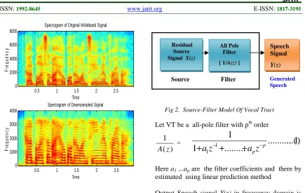
WB speech signal is shown in Fig 1 (top) and the corresponding NB representation is shown in Fig 1 (bottom ) . In the NB , high frequency components of above 4kHz is missing. In the recording , even the WB signal above 8 kHz is almost absent. It shows that , in the WB spectrum. the first harmonic components of the band 3.4kHz. to 4 kHz is also missing (above 7 kHz ). Here the challenging task will be the Creation of missing components between 4kHz. to 8 kHz

Generate an artificial WB sound form the NB sound using ABE techniques at the receiving end. Normally from the learned mutual relationship between the upper and lower frequency regions , the ABE techniques will create the missing frequency components . In this work , by

Time

F

re

q

u

e

n

c

y

Spectogram of Original Wideband Signal

0.5 1 1.5 2 2.5

0 2000 4000 6000 8000

Time

F

re

q

u

e

n

c

y

Spectogram of Downsampled Signal

0.5 1 1.5 2 2.5

0 1000 2000 3000 4000

Fig 1. WB And NB Signal

1.2.Previous Works

Schitzier (1998) gives a solution to reduce the bitrates for coding wideband speech, is to code the parameters of wider bandwidth speech with significant increase in bitrates relative to NB coders. Makhoul and Benarti (1979), Carl and Heute (1994), Yoshida and Abe (1994), Jax and Vary (2000) were discussed another approach that employ the WB enhancement by analysis and synthesis model. This technique synthesis the WB speech from the Pitch, Voicing , and spectral envelope information of NB speech. Many ABE methods, e.g. codebooks [2,3] , linear mapping [4] , Neural Networks etc is used to estimate the missing components. Again Jax and Vary [6, 7] found the potential features of speech and evaluate their performance for BWE application.

This paper organized as , in section II investigate the proposed methodology. The design of the proposed source filter modeled ABE is to be discussed in Section III , Section IV convolutes the results , Section V wrap up its performance and the upcoming work.

2. SOURCE-FILTER MODEL (VOCAL

TRACT) OFSPEECHPRODUCTION

The Vocal tract assumed as all pole filter. Speech generation can be modeled by source-filter model of VT and this is shown in Fig 2.

Fig 2. Source-Filter Model Of Vocal Tract

Let VT be a all-pole filter with pth order

)

(

1

z

A

=

...

...(

1

)

...

1

1

1 1

p p

z

a

z

a

+

+

+

Here a1 ...ap are the filter coefficients and there by

estimated using linear prediction method

Output Speech signal Y(z) in frequency domain is formed by multiplication of residual/source signal

X(z) by the VT all-pole filter 1/A(z) or by filtering X(z) by 1/A(z) in Time domain .

Y(z) = X (z) / A(z) --- (2)

A(z) can be obtained by using the filter coefficients a1 ...ap

X(z) = Y(z) A(z) --- (3)

In this source-filter model , we model the speech as a mixture of a sound source ( from vocal cords) ,then a linear acoustic filter, ( VT radiation characteristic). An important assumption is that the source and filter are independence each other.

Different phonemes can be distinguished by varying degrees, properties of their source(s) and their spectral shape. Voiced sounds (e.g., vowels) have source due to periodic glottal excitation. They can be easily approximated by an impulse train in time domain (TD) or harmonics in frequency domain (FD), and a filter that depends on position of tongue and protrusion of lip. Otherwise , fricatives have a source due to turbulent

noise. So called voiced fricatives such as "z" and "v" have two sources - one is at the glottis and another one is at the supra-glottal constriction.

Residual Source Signal X(z)

All Pole Filter

[ 1/A(z) ]

Speech Signal

Y(z)

Source Filter Generated

397 20 40 60 80 100 120 140 160 180 200 220 240 -0.5

0 0.5 1

Input signal and error signal(frame:26)

Samples[n]

A

m

p

lit

u

d

e

Inputsignal Inputsignal*hamming Errorsignal

0 500 1000 1500 2000 2500 3000 3500 4000

-80 -60 -40

FFT of input signal(frame:26) and frequency reponse of LPC

Frequency[Hz]

A

m

p

lit

u

d

e

[d

B

] FFT(fftpoints:512)

LPC(order:10)

One frame of a (20ms) given input NB signal (red) is taken. From the above relationship its corresponding Error /source (blue) is calculated and shown in Fig 3a (Top). Fig.3b (bottom) shows the FD representation (FFT spectrum shown in blue) of the TD signal frame and its corresponding Linear Prediction coefficients (red).

3. MODELING THE ARTIFICIAL BANDWIDTH EXTENTION SYSTEM

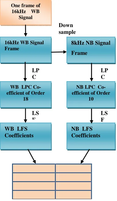
3.1. LSF Code Book Construction :

Construction of the LSF codebook is an important step in ABE system. Some training audio files are taken and separated in to uniform signal frames of 20 ms window size. For NB

speech 10th order Line Prediction Coefficient

(LPC) and for WB speech 18th order is used . For

quantization purpose LSF coefficients of WB representation of the signal frames and the LSF coefficients of down sampled NB representation of the corresponding signal frames are calculated.

Anb(z) = [ a1 , a2, a3, ………a10] --- (4)

The redundant entries in the code book can be minimized by applying clustering method. In our implementation, we didn’t use any clustering

algorithm since small set frames are used as training samples. The codebook stores NB-WB representation pairs and it is used in extension/filter phase, while assessment of

appropriate WB representation for the spectral envelope based on the available NB representation.

Fig 4. Lsf Codebook Construction

3.1.1. Linear predictive coding (LPC)

In audio / speech signal processing for representing the spectral envelope of a digital speech signal in compact form ( with less coefficients), LPC method is used ,with the information of a LP model.

3.1.2. Line Spectral Frequencies (LSF).

Various alternate useful representations are there for predictor coefficients. One of the most

important is Line Spectrum Pairs . In speech coding applications , LP polynomial of A(z) can be decomposed into LSF and this LSFs have a fine quantization and also interpolation properties Algorithm for the construction of the LSF codebook (CB) shown in Fig.4.

16kHz WB Signal Frame

8kHz NB Signal

Frame Down sample

WB LPC Co-efficient of Order

18

NB LPC Co-efficient of Order

10 LP

C

LP C

LS F

WB LFS Coefficients

NB LFS Coefficients

LS F One frame of

398

1. The WB FIR pre-emphasis filter has the

transfer function H (z) = 1 - 0.95z-1 shown in

Fig 5 was applied on the wideband training data wave files.

2. The NB signals are formed by down sampling

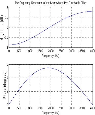
(decimating) the same WB training data wave files. Apply a suitable NB pre-emphasis filter shown in Fig 6 on the NB signals.

3. WB signal is Split in to frames of uniform

20ms window size with no overlap between adjacent frames . Then WB LPC as well as

equivalent WB LSF coefficients were

calculated.

4. Similarly NB signal is Split in to frames of

uniform 20ms window size with no overlap between adjacent frames . Then NB LPC as well as equivalent NB LSF coefficients were calculated..

5. Save the WB LSF coefficients beside with the

corresponding NB LSF coefficients .

3.2. Artificial Bandwidth Extention (ABE)

Each frame of NB signal is decomposed into two parts as a source part and a filter part and they are extended separately. The source signal is estimated by the filter coefficients using LP. The VT model is extended by the most appropriate WB model taken from a CB and the residual signal by TD zero-insertion method. Then the created signal is added to a delayed version of resampled original NB signal to structure an artificial WB signal.

ABE Steps :

The basic idea of ABE is to create a signal which contains the frequencies that are missing from the original NB signal . The algorithm for Source-filter based VT model is shown in Fig 7.

0 1000 2000 3000 4000 5000 6000 7000 8000 0 20 40 60 80 Frequency (Hz) P h a s e ( d e g re e s )

0 1000 2000 3000 4000 5000 6000 7000 8000 -30 -20 -10 0 10 Frequency (Hz) M a g n it u d e ( d B )

The Fequency Response of the Wideband Pre-Emphasis Filter

Fig 5. Frequency And Phase Response Of WB Pre-Emphasis Filter

0 500 1000 1500 2000 2500 3000 3500 4000 0 2 4 6 Frequency (Hz) P h a s e ( d e g re e s )

0 500 1000 1500 2000 2500 3000 3500 4000 -1 -0.5 0 0.5 1 Frequency (Hz) M a g n it u d e ( d B )

The Fequency Response of the Narrowband Pre-Emphasis Filter

Fig.6 Frequency And Phase Response Of NB Pre-Emphasis Filter

399

3.2.1. Spectral envelope extension / Filter part extension

1. The input NB signals which is to be extended is opened and a appropriate NB pre-emphasis filter was applied on the NB signals.

Xnb(z) = Ynb(z)Anb(z) --- (5)

2. The sampling rate of the NB signal is increased

using sample rate conversion . This will create a signal of spectrum 4-8kHz .

3. The LP coefficients of each NB frame is

calculated and Convert all LPC in to into LSFs.

4. Use the same window function which is used

in analysis phase, while constructing the LSF CB.

5. Find the NB CB entry with the minimum

Euclidean distance to the present LSF vector.

6. Get the equivalent WB LSF coefficients and

then exchange into LP coefficients for waveform synthesis

3.2.2. Source signal extension

7. Calculate the source/error signal using the NB

signal frames and its LPC coefficients

8. NB source signal is extended using rate

conversion technique (Xwb ).

9. Using the extended source signal (Xwb ) from

(8), and the WB LPC from (6) calculate the output signal.

10. Using overlap-add technique the extended

frames from (9) are concatenated. Here an analysis window of 20ms , synthesis window of 10ms and the time difference between adjacent frames is 5ms are used in both analysis and synthesis.

11. The signal from (10) were added/mixed with

the delayed version of NB resampled signal to get the final output.

Fig 8 top shows an example of 10th order NB LPC

coefficients and the Fig 8 bottom shows its corresponding spectral envelope

0 1 2 3 4 5 6 7 8 9 10

-4 -2 0 2

LPC coefficients (LPC order:10,Frame:26 of arctic_a0006.wav)

Coefficients[n] A m p lit u d e

0 500 1000 1500 2000 2500 3000 3500 4000 -100

-80 -60 -40 -20

LPC frequency response (frame:26 of arctic_a0006.wav)

Frequency[Hz] A m p li tu d e [d B ]

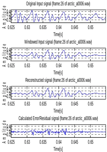
Fig 9 shows a original sample from (first) and its windowed version of signal(second). The third is the reconstructed NB signal

0.625 0.63 0.635 0.64 0.645 0.65 -0.20

0.2 0.4

Original Input signal (frame:26 of arctic_a0006.wav)

Time[s] A m p li tu d e

0.625 0.63 0.635 0.64 0.645 0.65 -0.20

0.2 0.4

Windowed Input signal (frame:26 of arctic_a0006.wav)

Time[s] A m p li tu d e

0.625 0.63 0.635 0.64 0.645 0.65 -0.20.20

0.4

Reconstructed signal (frame:26 of arctic_a0006.wav)

Time[s] A m p li tu d e

0.625 0.63 0.635 0.64 0.645 0.65 -0.20

0.2 0.4

Calculated Error/Residual signal (frame:26 of arctic_a0006.wav)

Time[s] A m p lit u d e

Fig 9. Different types of TD frames Fig 8. NB LPC coefficients and its

401

4. RESULTSANDDISCUSSION

The Speech Database

Carnegie Mellon University ARCTIC database by SLT (CMU ARCTIC SLT 0.95) contains (1132 utterances) a recording of the phonetically balanced US English speech by a female US English speaker. The speaker is experienced in building synthetic voices.

Table 1. MOS Scores and their Meaning

4.1 Performance Evaluation

We used two methods for evaluating the performance of the ABE techniques. One is comparing the spectrograms of extended signal with the spectrograms original wideband signal and the another is Mean Opinion Score.

4.1.1 Visualization using Spectrogram

Spectrogram, is a visual demonstration of sound. Since it is based on real measurements of the varying frequency component of a sound with time, spectrogram provides more absolute and precise information.

4.1.2. Mean Opinion Score (MOS)

For subjective measure, MOS preference test is conducted between the Original NB Signal, the interpolated version of NB signal and the ABW Extended version of signal. The objective of this test is to find which signal has the more hearable or understandable high frequency component sounds such as “sh”. We selected 10 NB files in which the high frequency components are almost absent but present in the corresponding original WB signals.

The NB signal, TDI version , and the ABWE signals were presented to 10 listeners (5 females

and 5 males) between 21 and 25 years of age having no auditory disorders were involved in the test. All the listeners had adequate knowledge on English and Phonetics for understanding all the given English speech signals/files.

For each listener the test was arranged individually in a quiet room using a simple graphical user interface ( GUI) on a computer screen. Through high quality headphones, test sample files were played on both ears of each listener. Before itself , the listeners had a little practice session.. During the practice session. the listeners can be allowed to adjust the volume setting to a suitable level. The arithmetic mean of all the individual scores is MOS, and generally its range is from 1 for worst case to 5 for best.

The values do not need to be whole numbers. Certain thresholds and limits are often expressed in decimal values from this MOS spectrum. For instance, a value of 4.0 to 4.5 is referred to as toll-quality and causes complete satisfaction. generally, the values dropping below 3.5 are termed unacceptable by many users.

4.2.1.Comparison of Resultant Spectrogram

M O S

Quality Impairment

5 Excellent Imperceptible

4 Good Perceptible but not annoying 3 Fair Slightly annoying

2 Poor Annoying

The spectrogram of conventional TDI BWE algorithm shown in Fig 10 (middle) had no signal components around 3.6 kHz to 4kHz and above 7.6 kHz. This is due to gain mismatch. Even Though it was mitigated it affect the quality of speech .These results implied that the proposed BWE algorithm created a frequency components around 3.6 kHz to 4kHz shown in Fig 10(c) a nd it could provide better quality of WB speech than the TDI BWE algorithm

4.3 Comparison of MOS

4.4 Observations :

Based on our observations, the selection pre-emphasis filters of WB and NB played an major role on extended speech quality . In the same way, the post- emphasis filter played an significant role on speech quality. It may have a great influence on changing the pitch of the original signal.

Analysis window size and synthesis window size also have an influences on the generated quality of speech .The number of WB LPC decides the final speech quality.

As we realized, the overall quality of the system will depend upon the LSF code book size. For better reproduction/bandwidth extension, we will need considerably LSF big code book. The increase in code book size will result in increase in overall delay.

5. CONCLUSION

In this paper, we designed the Source-filter model based on vocal tract and implemented ABWE algorithm using LPC coefficients. From the Spectrogram comparison, our proposed algorithm can able to represent consonant sounds, mostly fricative consonants ( th /, sh/, / Isl /, xl/ ch, /, etc). Artificial Band Extension (ABE) techniques are used to generate a wideband signal from the

Audio

File

Mean Opinion Score

Origin

al NB

Signal

Inter

polated

WB

Signal

ABE WB

Signal

1

3.00

3.05

4.00

2

3.00

3.40

4.00

3

3.25

3.50

4.50

4

3.00

3.75

4.00

5

3.00

3.50

4.25

6

3.25

3.00

4.75

7

3.00

3.25

4.50

8

3.00

3.50

4.50

9

3.00

3.73

4.25

10

3.00

3.50

4.00

Avg.

3.05

3.463

4.275

Fig. 10. Spectrogram Comparison.

Table 2. Mean Opinion Score of Different Listeners

.

403 narrowband signal. The spectrogram of extended signals shows the obvious creation of missing bands. The performance MOS preference test proved that from the NB signal the ABE system created almost the original WB signal. In most of the practical system, the WB signal will be available at the transmitting end and before transmission, it will be converted in to NB signal to minimize transmission cost (narrowband channel is only available). In such cases, the wideband LPC coefficients can be directly transmitted along with the NB signal. So that, at the receiving end, instead of maintaining a codebook, the bandwidth extension can be done by directly using the WB LPC coefficients. For that we may use data hiding technique, inside each signal frame itself , to hide

the corresponding WB LPC coefficients.

Steganography based data hiding ABE system will not effect the existing transmission and reception methods very much. Even a standard receiving system may play the narrowband signal as it is without processing the hidden LPC coefficients. Our future works will concentrate on the ways to implement such an efficient Steganography based ABE systems.

ACKNOWLEDGEMENT

This work was supported by Periyar Maniammai University . This work has successfully completed by the active support of Prof. S.Jayakumar Dean SCSE, and Prof. D.kumar Dean Research , PMU.

REFERENCES

[1] Carl,H., and Heute,U., 1994 “Bandwidth Enhancement of narrow band speech

signals”, Signal Processing VII,

Theories and applications, EUSIPCO, Vol 2, pp. 1178- 1181.

[2] CCITT, 1988 ,“7 kHz Audio Coding Within 64 kBit/s”, Recommendation G.722, Vol. Fascile III.4 of Blue Book, Melbourne.

[3] Cheng,Y.M., ’Shaughnessy,D.O,

Mermelstein,P., 1994 “Statistical Recovery of

Wideband Speech from Narrowband

Speech”. IEEE Transactions on Speech and Audio Processing, vol.2, no4,pp.544– 548. [4] Chennoukh,S., Gerrits, A., Miet, G.,and

Sluitjer, R., May 2001 "Speech enhancement via frequency bandwidth extension using line spectral frequencies," Pro. IEEE Int.

Conf. On Acoustics, Speech, Signal

Processing, vol. 1, pp. 665- 668.

[5] 3GPP TS 26.171, March 2001 “Speech Codec speech processing functions; AMR WB Speech Codec; General Description”. Version 1.

[6] Gandhimathi,G., Narmadh,C., and Lakshmi,C. August 2010 ,” Simulation of Narrow

Band Speech Signal using BPN

Networks “ , International Journal of Computer Applications (0975 - 8887) Volume 5- No.9.

[7] Gandhimathi.G., Jayakumar,S.,2013,“Speech

enhancement Using Artificial Bandwidth

Extension Algorithm in

Multicast conferencing throughCloud services, Information Technology Journal , ISSN 5638 pp.1-8.

[8] Heide, D.A. , Kang, G.S., May 1998, "Speech enhancement for band limited speech", in Proc of the ICASSP, Vol. 1, Seattle, WA, USA, pp. 393-396.

[9] http://www.festvox.org/cmu_arctic/2003

Carnegie Mellon University, Copyright (c)

[10] Jax P., and Vary, P., 2000 “ Wide band Extension of speech using Hidden Markov Model” in Proc. IEEE workshop on speech coding .

[11] Jax P., and Vary, P., May 2002. "An upper bound on the quality of artificial bandwidth extension of narrowband

speech signals", Pro. IEEE International

Conference on Acoustics, Speech, and Signal Processing (ICASSP) vol. 1, pp 237- 240, Orlando, FL, USA.

[12] Jax P., and Vary, P., May 2004., "Feature

Selection for Improved Bandwidth

Extension of Speech Signals", Pro.IEEE

International Conference on Acoustics,

Speech, and Signal Processing (ICASSP) vol. 1, pp. 697-700, Montreal, Canada.

[13] Makhoul, J., Berouti,M., 1979,” High frequency generation in speech coding system “, in proc. ICASSP, pp 428-431. [14] Miet, G., Gerrits, A., and Valiere, J. C., Jun

2000., "Low-band extension of

telephone-band speech," Pro.

IEEE Int. Conf. On Acoustics, Speech, Signal Processing, vol. 3, pp. 1851-1854.

[15] Park, K.-Y., Kim,. H. S. June 2000 “Narrowband to Wideband Conversion

of Speech using GMM-based

[16] Qian, Y. and Kabal, P., May 2004 "Combining Equalization and Estimation for Bandwidth Extension of Narrowband Speech", Proc. IEEE Int. Conf. Acoustics, Speech, Signal Processing (Montreal, QC), pp. 1-713-1-716.

[17] SchnitZier,J. 1998 ,” A 13.0 Kbit/S wide band codec based on SB- ACELP”, in Proc.ICASSP, Vol.1, pp-157- 160 [18] Yoshida ,Y.,and Abe ,M., 1994 ,”An