A LIMITED MEMORY BFGS ALGORITHM WITH SUPER
RELAXATION TECHNIQUE FOR NONLINEAR
EQUATIONS
1GONGLIN YUAN, 2ZENGXIN WEI, 3YONG LI, 4XUPEI ZHAO
1
Prof., College of Mathematics and Information Science,Guangxi University,Gonglin Yuan
2Prof., College of Mathematics and Information Science,Guangxi University,Zengxin Wei
3 Assoc. Prof.,Department of Mathematics, Baise University,Yong Li
4 Master Student., College of Mathematics and Information Science,Guangxi University, Xupei zhao
E-mail: [email protected], [email protected],
3 [email protected], 4[email protected]
ABSTRACT
In this paper, a trust-region algorithm combining with the limited memory BFGS (L-BFGS) update is proposed for solving nonlinear equations, where the super relaxation technique(SRT) is used. We choose the next iteration point by SRT. The global convergence without the nondegeneracy assumption is obtained under suitable conditions. Numerical results show that this method is very effective for large-scale nonlinear equations problems.
Keywords: Algorithm; L-BFGS Update; Super Relax; Nonlinear Equations.
1. INTRODUCTION
Consider the following system of nonlinear equations:
( ) 0, n,
g x = x∈ ℜ (1.1)
Where g:ℜ → ℜn nis continuously differenti- able. The problem (1.1) has many applications in engineering, such as nonlinear fitting, function approximating and parameter estimating.
There are many algorithms that have been proposed for (1.1), for examples, Gauss- Newton method [1, 8, 12, 14], Levenberg-Marquardt method [5, 20, 31], trust region method [4, 21], and quasi-Newton method [7, 32], etc.. If the Jacobian matrix ∇g x( ) of
g x
( )
is symmetric for alln
x∈ ℜ , then this problem is called symmetric nonlinear equations. Li and Fukushima[9,10] presented Gauss-Newton-based BFGS methods to solve it. These years we made a further study and got some results (see [22, 23, 25, 26, 27, 28, 30]).
Let ϕ be the norm function defined by
2 1
2
( )x || ( ) || .g x
ϕ = Suppose that
g x
( )
has a zero,then the nonlinear equation problem (1.1) is equivalent to the following global optimization problem
min ( ),ϕ x x∈ℜn. (1.2)
The trust region method is one of the effective methods for the above problem, where the traditional trust region methods, at each iterative point
x
k, the trial stepdkis obtained by solving the
following trust-region subproblem
Minimizep d such that k( ) d ≤ ∆, (1.3)
where 1 2
2
( ) ( ) ( )
k k k
p d = g x + ∇g x d . The trust region methods are globally and superlinearly convergent under the condition that ∇g x( ∗)( x∗ is a solution of (1.1)) is nondegenerate, where nonde- generacy means nonsingularity. Nondegeneracy of
( )
g x∗
∇ seems a too stringent requirement for the purpose of ensuring superlinear convergence. Then Zhang and Wang [31] give a new trust region method:
Minimize φk( )d such that cp g x( k)γ, (1.4)
where 1 2
2
( ) ( ) ( ) , 0 1,
k d g xk g x dk c p
φ = + ∇ < < is
a non- negative integer, and 0.5< <γ 1.
the local error bound condition which is weaker than the nondegeneracy assumption [see [20]]. However, the global convergence also need the nondegeneracy of ∇g x( ∗). Presently, there is no algorithm which has the property that the iterative sequence generated by the algorithm can satisfy
( k) 0
g x → . Without the assumption that ∇g x( ∗)
is nondegenerate. In order to overcome this drawback, Yuan et al. [27] presented the trust region subproblem
Minimizeh d such that k( ) d ≤ ∆k, (1.5)
Where 1 2
2
( ) ( ) ,
k k k
h d = g x +B d the radius of trust
region ∆kis defined by p ( )
k c g xk
∆ = , c∈(0, 1),
p
is a nonnegative integer, andB
kis generated by BFGS formula. Comparing with the first two methods, the third method uses the BFGS update matrix instead of the Jacobian matrix. It is well known that the trust-region method will be very useful with the situation when the exact Jacobian or Hessian computation is inexpensive or possible. However, this case is very inferquent in many practices. Then the third trust region method is more efficient than the first two methods for normal practical problems. However, all of these three methods need to store and compute the matrix (the Jacobian or the BFGS update matrix) at every iterations in the algorithm. It can clearly increase the storage and workload in computation, especially for large-scale problems. One of the effective methods to overcome this insufficient is reducing the matrix term. In this paper, we give a trust region method based on the method of [27] which does not compute and store the matrix completely.Limited memory quasi-Newton methods are known to be effective techniques for solving certain classes of large-scale unconstrained optimization problems (see Buckley and Le Nir [3], Liu and Nocedal [11], Gilbert and Lemar´echal [6], and Byrd, Nocedal, and Schnabel[2]). They make simple approximations of Hessian matrices, which are often good enough to provide a fast rate of linear convergence, and require minimal storage. The implementation is almost identical to that of the standard BFGS method, the only difference is that the inverse Hessian approximation is not formed explicitly, but defined by a small number of BFGS updates. Thus it often provides a fast rate of convergence and requires minimal storage. Some authors have made a study about this technique (see [15, 18, 19, 24, 28, 29] etc.).
Inspired by the above observations, we present a new method, which not only possesses the global convergence without the nondegeneracy assumption under suitable conditions, but also does not compute the matrix completely at every iterations. Naturally, we use limited memory quasi-Newton update matrix instead of the normal matrix (the Jacobian or the quasi-Newton matrix). The given algorithm has the following attributes.
•the matrix of the trust region subproblem is generated by limited memory quasi-Newton update.
•the the next iteration point is determined by super relaxation technique.
•the global convergence without the nondegen- eracy assumption under suitable conditions is established.
• numerical results show that the given algorithm is very effective for largescale problems.
Here and throughout this paper, we use the following notations. . Denote the Euclidian norm
of vectors or its induced matrix norm, andg x( k)is replaced byg . k
This paper is organized as follows. In Section 2, the algorithm is represented. In Section 3, we prove some convergent results. The numerical results of the method are reported in Section 4.
2. MOTIVATIONS AND ALGORITHM
In this section, we will introduce the limited memory BFGS (L-BFGS) method and the super relaxation technique (SRT) respectively. Then we give the proposed algorithm.
2.1 The limited memory BFGS method
The L-BFGS method is an adaptation of the BFGS method to large-scale problems. The implementation described by Liu and Nocedal [11] is almost identical to that of the standard BFGS method-the only difference is in the matrix update, for getting Hessian inverse approximate Hk+1 , instead of storing matrices H , at every iteration k
k
x
the method stores a small number, say m, of correction pairs{ ,s yi i}, i= −k 1,K,k−m,where1
1
,
.
k k
k k k k
s
=
x
+−
x y
=
g
+−
g
ained case indicating the limited memory BFGS
performs well. Let k 1
T
k k
y s
ρ = and T.
k k k k
U= −I
ρ
y s Ifwe use the stored correction pairs, then
[
]
1
1 1 1 1 1 1
1 1 1 1 1 1
1 1 1 1 1
2 1 1 2 1
( )
[ ] [
] [ ]
k
T T T T
k K k k k k k k k k k
T T T T T
k k k k k k k k k k k k
T T T
k k m k m k m k k m k
T T T
k m k m k m k m k k k k
H
U U H U s s U s s
V U H U U s s U s s
U U H U U U
U s s U U s s
ρ ρ
ρ ρ
ρ ρ
+
− − − − − −
− − − − − −
− + − + − + + − −
− + − + − + − + −
= + +
= + +
=
= +
+ +
L
L L
L L L
(2.1)
Wheresk =xk+1−xkandyk g x(k1, k1) g x( , )k k
α ε α ε
+ +
= −
To maintain the positive definiteness of the L-BFGS matrix, some researches discard a correction pair [ ,s yk k]if the curvature 0
T k k
s y > is not satisfied (see
[18]). Another approach was proposed by Powell [17] where
y
kis defined by, 0.2
(1 ) , ,
T T
k k k k k k
k
k k k k k
y if s y s B s
y
y B s others
θ θ
≥
=
+ −
(2.2)
Where 0.8T
k k k
k T T
k k k k k
s B s
s B s s y
θ =
− and
1
( ) .
k k
B = H −
2.2 The Super Relaxation Technique
The super relaxation technique (SRT) is often used in computation mathematics to improve the accuracy, where two target values are generally chosen as a weighted average. The heart of the super relaxation technique is the development of advantage and the inhibition of inferior in the relaxation process, where the relaxation factor plays an important role. However, this technique is rarely used in numerical optimization methods. In the algorithm of this paper, we will use the SRT to improve the efficiency for large scale nonlinear equations.
Based on the above discussions, the given L-BFGS trust region subproblem is defined by
Minimizeq d such that k( ) d ≤ ∆k, (2.3)
Where 1 2
2
( ) ( ) ,
k k k
q d = g x +B d the radius of trust
region ∆k is defined by p
k c
∆ = g x( k) ,
(0,1),
c∈ pis a nonnegative integer, and 1
k k
B =H− is
generated by the L-BFGS formula (2.1) andB0is an
initial symmetric positive definite matrix. Letd be kp
the solution of (2.3) corresponding to p , and
letx be the kth iteration point. Then the next point k
is defined by the SRT. (1) Updated point:
1 .
d p
k k k
x+ =x +d (2) Super relaxation point:
1 (1 ) 1, [0,1]
d
k k k
x+ =wx + −w x+ w∈ is the super
relaxation factor.
According to the new trust region subproblem (2.3) and the above super relaxation point, we define the actual reduction as
( p) ( p) ( ),
k k k k k
Ared d =ϕ x +d −ϕ x (2.4)
and the predict reduction as
Pr ( p) ( p) (0).
k k k k k
ed d =q d −q (2.5)
Now we the algorithm for solving (1.1) is given as follows.
• Algorithm 1.(L-BFGS trust region with SRT)
Initial: Given constants ρ,c∈[0,1] w∈[0,1],
0
0, 0, n,
p= ε> x ∈ℜ 1
0 0
n n
B =H− = ∈ℜ × ℜI is
symmetric and positive definite. Let k := 0;
Step 1: If gk <ε, stop. Otherwise, go to step 2;
Step 2: Solve the trust region subproblem (2.3)
with∆ = ∆kto get d ; k
Step 3: Calculate ( p)
k k
Ared d ,and the radio of actual reduction over predict reduction as
(
)
.
Pr
(
)
p
p k k
k p
k k
Ared
d
r
ed
d
=
(2.6)If p ,
k
r <ρ then we let p = p + 1, go to step 2. Otherwise, go to step 4;
Step 4: Let d1 p,
k k k
x+ =x +d 1 (1 ) 1,
d
k k k
x+ =wx + −w x+
1
k k k
y =g+ −g , update 1
1 1
k k
H+ =B−+ by (2.1).
Step 5: Set k := k + 1 and p = 0. Go to step 1.
Remark. (i) In this algorithm, the procedure of
“Step 2-Step 3-Step 2” is named as inner cycle.
(ii) In order to ensure the update matrix Hk
generated by (2.1), the technique (2.2) of [17] is used.
(iii) In Step 4, if w=0, then 1 d1
k k
x+ =x+ =
, p
k k
x +d the given algorithm is the normal L-BFGS
trust region algorithm.
3. CONVERGENCE ANALYSIS
we also give the detail proof.
Lemma 3.1 If d is the solution of (2.3), then kp
2
1
P r ( ) m in { , } . 2
k k p
k k k k k
k B g e d d B g
B
− ≥ ∆ (3.1)
Proof. Since p
k
d is the solution of (2.3), for any
[ ]
0,1 ,α ∈ we get
2 2
2
2 2
P r ( ) P r ( )
1
( )
2 ( ) /
1
.
2
p k
k k k k k
k k
T
k k k k k k k
k k k k k
k k k k k k
e d d e d B g
B g
B g B B g
B B g B g
B g B B
α
α α
α α
∆
− ≥ − −
= ∆ − ∆
≥ ∆ − ∆
Thus, we have
2
2 2
0 1
2
1
Pr ( ) max[ ]
2 1
min{ , }. 2
p
k k k k k k k
k k
k k k
k
ed d B g B
B g B g
B
α α α
≤ ≤
− ≥ ∆ − ∆
≥ ∆
The proof is complete.
In order to get the global convergence, similar to [27, 31], the following assumption conditions are needed.
Assumption i (A) Let the level setΩ
0 {xϕ( )x ϕ(x )}
Ω = ≤ (3.2)
be bounded.
(B) g x is twice continuously differentiable on ( ) an open convex setΩ1containingΩ. The normal
function ( ) 1|| ( ) ||2
2 k
x g x
ϕ = is descent along the
direction p, ., k
d ie
( )T p 0.
k k
x d
ϕ
∇ ≤ (3.3)
(C) The following relation
[∇g x( k)−B gk] k =O d( kp ) (3.4)
Holds.
(D) The matrices{Bk}are uniformly bounded
on Ω1 ,which means that there exist positive constants0<M0 ≤M and 0<m1such that
1
0 k , k 1
M ≤ B ≤M B− ≤m ∀k. (3.5)
Assumption i(B) implies that there existsM1 >0
such that
( )T ( ) 1, .
k k
g x g x M k
∇ ∇ ≤ ∀ (3.6)
Similar to [27], we have the following two lemmas, here we only state them but omit the proof.
Lemma 3.2 (Lemma 3.1 of [27]) If d is the kp
solution of (2.3). Let Assumption
i
holdand{ }xk be generatedby Algorithm 1. Then
2
( p) Pr ( p) ( p ).
k k k k k
Ared d − ed d =O d
Lemma 3.3 (Lemma 3.2 of [27]) Let Assumption
ihold and { }xk be generated by Algorithm 1. Then Algorithm1 does not circle in the inner cycle infinitely.
Lemma 3.3 shows that the proposed algorithm is well-defined.
Lemma 3.4 Let Assumption i hold and{ }xk be
generated by Algorithm 1. Then{ }xk ⊂ Ω. More- over, { (ϕ xk)}converges.
Proof. By Taylor formula and (3.3), we have
1
( ) ( ) [ (1 )( )] ( )
(1 ) ( ) ( ) 0
p
k k k k k k
T p p
k k k
x x wx w x d x
w x d o d
ϕ ϕ ϕ ϕ
ϕ
+ − = + − + −
= − ∇ + ≤ (3.7)
The above relation implies that
ϕ
(
x
k+1)
≤
ϕ
(
x
k)
0
(x )
ϕ
≤L≤ . Then we conclude that { (ϕ xk)}
converges. The proof is complete.
Similar to [27], we have the global convergence, here state it and give the proof process as follows. The following theorem says that the iterative sequence { }xk generated by Algorithm 1 satisfies
|| ( ) ||g xk →0 without the assumption that
*
( )
g x
∇ is
nondegenerate, where x is a cluster point of * { }xk .
Theorem 3.1 Let Assumption i holds, { }xk be
generated by the Algorithm 1. Then the algorithm either stops finitely or generates an infinite sequence{ }xk such that
lim || k || 0.
k→∞ g = (3.8) Proof. If the algorithm does not stop finitely, suppose that the relation
lim || k k || 0
1 1
1
0 ||≤ gk || ||= B B gk− k k|| ||≤ Bk− ||||B gk k ||≤m ||B gk k ||, then we can get (3.8). Thus, in order to complete this lemma, we only to obtain (3.9).Assume, on the contrary, that there exists a constant ε >0and an subsequence{ }kj such that
|| ||
j j
k k
B g ≥ε (3.10)
Define the index setK={ | ||k B gk k||≥ε}. Mean-
while, by Assumption i and||B gk k||≥ε,(k∈K),||gk||
(k∈K)is bounded away from 0. Without loss of generality, we can assume||gk ||≥ ∀ ∈ε, k K.
By Lemma 3.1 and the definition of Algorithm 1, we have
2
1
[ ( ) ( )] . Pr ( )
2
. min{ , }. ,
k
k
p p
k k k k k
k K k K
p
k K
x x d ed d
c M
ϕ ϕ ρ
ε
ρ ε ε
∈ ∈
∈
− + ≥ −
≥
∑
∑
∑
wherepkis the largest
p
value obtained in the inner circle at the iterative pointxk.Lemma 3.4 shows that{ (ϕ xk)}is convergent,
then the following relation
2
1
. min{ , }.
2
k
p
k K
c M
ε
ρ ε ε
∈
< +∞
∑
holds. Thus, pk → +∞ask→ +∞ andk∈K .
Then we assume that
p
k≥
1
for all k∈K.Using the determination of p kk( ∈K) in the
inner circle, the solution
d
k′
corresponding to the following subproblem2
1
1
min ( ) || ( ) ||
2
. . || || k || ||,
k k k
p k
q d g x B d
s t d c − g
= +
≤
(3.11)
is unacceptable. Letxk′+1 =xk +dk′, we get
( ) ( 1)
. ( )
k k
k k
x x
Pred d
ϕ −ϕ ′+ <ρ
′
− (3.12)
From Lemma 3.1, we have
1 2
1
( min{ , }. .
2 k
p
k k
Pred d c
M ε
ε ε
−
′
− ≥
By Lemma 3.2, we obtain
1
2( 1) 2
( ) ( ) ( )
(|| || ) ( k ).
k k k k
p k
x x Pred d
O d O c
ϕ + ϕ
−
′ − − ′
′
= =
Therefore,
2( 1) 1
1 2
( ) ( ) ( )
| 1 | .
( )
0.5 min{ , }.
k
k
p
k k
p
k k
x x O c
Pred d
c M
ϕ ϕ
ε
ε ε
− +
−
′ −
− ≤ ′
Since pk → +∞ as k→ +∞ and k∈K , we have
1
( ) ( )
1, ,
( )
k k
k k
x x
k K
Pred d
ϕ −ϕ ′+ → ∈
′
− this contradicts (3.12).
This completes the proof.
4. NUMERICAL RESULTS
In this section, we report results of some large scale numerical experiments with the proposed method. We list the test functions as follows [16]
1 2
( ) ( ( ), ( ), ( ))T
n
g x = f x f x L f x ,
where these functions have the associated initial guessx0. Where A of Function 8 is the n×n tridiago- nal matrix given by
8 1 1 8 1
1 8 1
1 1 8
A −
− −
− −
=
−
−
O O O O O
In the experiments, the parameters were chosen asρ=0.0001,ε=10 ,−5 c=0.1, γ =0.7, w=0.2,
0
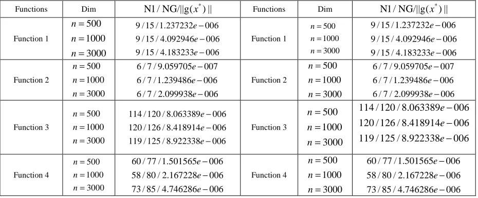
B is the unit matrix. We obtaindkby (2.3) from Dogleg method. In the inner circle of Algorithm 1, we will accept the trial step ifp>5 holds.We also stop the program if the iteration number is larger than fifteen hundred. The program was coded in MATLAB 7.0. The columns of the tables have the following meaning: Dim: the dimension of the problem. NG: the number of the norm function evaluations. NI: the total number of iterations.
*
( )
g x : the final function value at the last point.
From Table 2, we can see that our algorithm performs quite well from these problems, and the dimension does not influence the performance of the presented method obviously. For Problem 3 and Problem 7, we can see that the iteration number and the normal function number of dimension 3000 is less than those of dimension 1000.The reason maybe lie in that the number is limited(p≤5)in the inner cycle.
5. CONCLUSION
global convergence is established. The main work of this paper is extent the super relaxation to the
nonlinear equation problems, moreover, the
L-BFGS update is used to replace the matrix of the trust-region subproblem.
Table 1 (Test Functions)
1.Trigonometric function
1
( ) 2( (1 cos ) sin
cos )(2 sin cos ), 1, 2, 3, ,
i i i
n
j i i
j
f x n i x x
x x x i n
=
= + − −
−
∑
− = L0
101 101 101
( , , , ) .
100 100 100
T
x
n n n
= L
2.Logarithmic function ( ) ln( 1) i, 1, 2,3, ,
i i
x
f x x i n
n
= + − = L 0 (1,1, ,1) .
T
x = L
3.Broyden Tridiagonal function
1 1 1 2
1 1
1
( ) (3 0.5 ) 2 1,
( ) (3 0.5 ) 2 1, 2, 3, , 1,
( ) (3 0.5 ) 1.
i i i i i
n n n n
f x x x x
f x x x x x i n
f x x x x
− + −
= − − +
= − − + + = −
= − − +
L 0 ( 1, 1, , 1) .
T x = − − L−
4.Trigexp function
1
1
3
1 1 2 1 2 1 2
2
1 1
1 1
1
( ) 3 2 5 sin( ) sin( ),
( ) (4 3 ) 2
sin( ) sin( ) 8, 2, 3, , 1,
( ) 4 3.
i i
n n
x x
i i i i i
i i i i
x x
n n n
f x x x x x x x
f x x e x x x
x x x x i n
f x x e x
− − − − + + + − − = − − + − + = − − + + + − + − = − = − + − L 0
(0, 0, , 0) .T
x = L
5.Strictly convex function ( ) xi 1, 1, 2, 3, ,
i
f x =e − i= Ln 0
1 2 ( , , , ) .T
x n n = L 6.Variable dimensioned function 2 1 1 2 2 1
( ) 1, 1, 2, 3, , 2,
( ) ( 1),
( ) ( ( 1)) .
i i
n
n j j
n
n j j
f x x i n
f x j x
f x j x
− − = − = = − = − = − = −
∑
∑
L 0 1 2(1 ,1 , , ) .T
x
n n
= − − L
7.Discrete boundry value function
2 3
1 1 1 2
2 3
1 1
2 3
1
( ) 2 0.5 ( ) ,
( ) 2 0.5 ( ) , 2,3, , 1,
1
( ) 2 0.5 ( ) , .
1
i i i i i
n n n n
f x x h x h x
f x x h x hi x x i n
f x x h x hn x h n − + − = + + − = + + − + = − = + + − = +
L x0 =( (h h−1),L, (h nh−1)).
8.Discretized two-point boundry value function
2
1 2
1
( ) ( )
( 1)
( ) ( ( ), ( ), , n( )) ,T i( ) sin i 1,
g x Ax F x
n
F x F x F x F x F x x
= +
+
= L = −
0 (50, 0,50, 0, ).
x = L
Table 2 (Test results for Algorithm 1)
Functions Dim N1 / NG/||g(x*) || Functions Dim N1 / NG/||g(x*) ||
Function 1 500 1000 3000 n n n = = =
9 / 15 / 1.237232 006 9 / 15 / 4.092946 006 9 / 15 / 4.183233 006
e e e − − − Function 1 500 1000 3000 n n n = = =
9 / 15 / 1.237232 006 9 / 15 / 4.092946 006
9 / 15 / 4.183233 006 e e e − − − Function 2 500 1000 3000 n n n = = =
6 / 7 / 9.059705 007 6 / 7 / 1.239486 006 6 / 7 / 2.099938 006
e e e − − − Function 2 500 1000 3000 n n n = = =
6 / 7 / 9.059705 007 6 / 7 / 1.239486 006 6 / 7 / 2.099938 006
e e e − − − Function 3 500 1000 3000 n n n = = =
114 / 120 / 8.063389 006 120 / 126 / 8.418914 006 119 / 125 / 8.922338 006
e e e − − − Function 3 500 1000 3000 n n n = = =
114 / 120 / 8.063389 006
120 / 126 / 8.418914 006
119 / 125 / 8.922338 006
e e e − − − Function 4 500 1000 3000 n n n = = =
60 / 77 / 1.501565 006
58 / 80 / 2.167228 006 73 / 85 / 4.746286 006
e e e − − − Function 4 500 1000 3000 n n n = = =
60 / 77 / 1.501565 006 58 / 80 / 2.167228 006 73 / 85 / 4.746286 006
[image:6.612.69.534.519.712.2](i) Since the L-BFGS has a fast rate of convergence and requires minimal storage. Then the matrix of the trust region subproblem is generated by L-BFGS update.
(ii) In order to get better numerical results, the SRT is used in the algorithm where the next iteration point is determined by super relaxation technique.
(iii) Similar to \cite{yuan113}, the global convergence without the nondegeneracy assumption under suitable conditions is established.
(iv) In order to show the performance of the given algorithm, large-scale problems are tested. Practical results show that the given algorithm is effective.
ACKNOWLEDGMENT.
This work is supported by Guangxi NSF (Grant No. 2012GXNSFAA053002) and China NSF (Grant No. 11261006, 11161003 and 71001015).
REFERENCES
[1] D. P. Bertsekas, Nonlinear programming, Athena Scientific, Belmont, 1995.
[2] R. H. Byrd, J. Nocedal, and R. B. Schnabel, Representations of quasi-Newton matrices and their use in limited memory methods, Mathema- tical Programming,63(1994), pp. 129-156. [3] A. Buchley and A. LeNir, QN-like variable stor-
age conjugate gradients, Mathematical Program- ming, 27(1983), pp. 577-593.
[4] A. R. Conn, N. I. M. Gould, and P. L.Toint,Trust region method, Society for Industrial and Applied Mathema-tics, Philadelphia PA, 2000. [5] J. Y. Fan, A modified Levenberg-Marquardt
algorithm for singular system of nonlinear equa- tions, Journal of Computational Mathematics, 21(2003), pp. 625-636.
[6] J. C. Gilbert and C. Lemar´echal, Some numeri- cal experiments with variable storage quasi- Newton algorithms, Mathematical Programming, 45(1989), pp. 407-436.
[7] A. Griewank, The ’global’ convergence of Broyden-like methods with a suitable line search, Journal of the Australian Mathematical Society, Series B, 28(1986), pp. 75-92.
[8] K. Levenberg, A method for the solution of certain nonlinear problem in least squares. Quarterly of Applied Mathematics, 2(1944), pp. 164-166.
[9] D. Li and M. Fukushima, A global and super-
linear convergent Gauss-Newton-based BFGS method for symmetric nonlinear equations, SIAM Journal on Numerical Analysis, 37(1999), 152-172.
[10] D. Li, L. Qi, and S. Zhou, Descent directions of quasi-Newton methods for symmetric nonlin- ear equations,SIAM Journal on Numerical Analysis, (5)40(2002), pp. 1763-1774.
[11] D. C. Liu and J. Nocedal, On the limited memory BFGS method for large scale optimiza- tion, Mathematical Programming, 45(1989), pp. 503-528.
[12] D. W. Marquardt, An algorithm for leastsqu- ares estimation of nonlinear inequalities. SIAM Journal on Applied Mathematics, 11(1963), pp. 431-441.
[13] J. J. Mor´e, Recent development in algorithm and software for trust region methods, in: A. Bachem, M. Grotschel, B. Kortz (Eds.), Mathe- matical Programming: The State of the Art, Spinger-Verlag, Berlin, 1983, 258-285.
[14] J. Nocedal and S. J. Wright, Numerical optimization, Spinger, New York, 1999.
[15] Q. Ni and Y. Yuan, A subspace limited memory quasi-Newton algorithm for large-scale nonlin- ear bound consrtained optimization, Mathema- tics of Computation,66(1997), pp. 1509-1520. [16] J. M. Ortega and W. C. Rheinboldt, Iterative
solution of nonlinear equations in several variables, Academic Press, New York, 1970. [17] M. J. D. Powell, A fast algorithm for nonlin-
early constrained optimization calculations, Numerical Analyis, (1978), pp. 155-157. [18] R. H. Ryrd, P. H. Lu, J. Nocedal, and C. Y. Zhu,
A limited memory algorithm for bound constr- ained optimization, SIAM Journal on Scienti- fic Computing, 16(1995), pp. 1190-1208. [19] Y. Xiao and D. Li, An active set limited memory
BFGS algorithm for large-scale bound
constrained optimization, Mathematical Meth- ods of Operations Research, 67(2008), pp. 443-454.
[20] N. Yamashita and M. Fukushima, On the rate of
convergence of the Levenberg-Marquardt
Method, Computing, 15(2001), pp. 239-249. [21] Y. Yuan, Trust region algorithm for nonlinear
equations, Information, 1(1998), pp. 7-21. [22] G. Yuan, A new method with descent property
[23] G. Yuan and X. Lu, A new backtracking inexact
BFGS method for symmetric nonlinear
equations, Computers and Mathematics with Applications, 55(2008) pp. 116-129.
[24] G. Yuan and X. Lu, An active set limited memory BFGS algorithm for bound constrained optimization,Applied Mathematical Modelling, 35(2011), pp. 3561-3573.
[25] G. Yuan, X. Lu, and Z. Wei, BFGS trust-region method for symmetric nonlinear equations,
Journal of Computational and Applied
Mathematics, (1)230(2009), pp. 44-58.
[26] G. Yuan, S. Lu, and Z. Wei, A new trust-region method with line search for solving symmetric nonlinear equations, International Journal of Computer Mathematics, 88(2011), pp. 2109- 2123.
[27] G. Yuan, Z. Wei, and X. Lu, A BFGS trust-region method for nonlinear equations, Computing, 92(2011), pp. 317-333.
[28] G. Yuan, Z. Wei, and S. Lu, Limited memory BFGS method with backtracking for symme- tric nonlinear equations, Mathematical and Computer Modelling, 54(2011), pp. 367-377 [29] G. Yuan, Z. Wei, and Y. Wu, Modified limited
memory BFGS method with nonmonotone line search for unconstrained optimization, Journal of the Korean Mathematical Society, 47(2010), pp. 767-788.
[30] G. Yuan and S. Yao, A BFGS algorithm for
solving symmetric nonlinear equations,
Optimization,DOI:10.1080/02331934.2011.564 621.
[31] J. Zhang and Y. Wang, A new trust region method for nonlinear equations, Mathematical Methods of Operations Research, 58(2003), pp. 283-298.