http://www.scirp.org/journal/alamt ISSN Online: 2165-3348 ISSN Print: 2165-333X
A QMR-Type Algorithm for Drazin-Inverse
Solution of Singular Nonsymmetric
Linear Systems
Alireza Ataei
Department of Mathematics, Faculty of Science, Persian Gulf University, Bushehr, Iran
Abstract
In this paper, we propose DQMR algorithm for the Drazin-inverse solution of con-sistent or inconcon-sistent linear systems of the form Ax=b where A∈N N× is a
singular and in general non-hermitian matrix that has an arbitrary index. DQMR al-gorithm for singular systems is analogous to QMR alal-gorithm for non-singular sys-tems. We compare this algorithm with DGMRES by numerical experiments.
Keywords
Singular Linear Systems, DGMRES Method, Quasi-Minimal Residual Methods, Drazin-Inverse Solution, Krylov Subspace Methods
1. Introduction
Consider the linear system,
Ax=b (1)
where N N
A∈ × is a singular matrix and ind
( )
A is arbitrary. Here ind( )
A , theindex of A is the size of the largest Jordan block corresponding to the zero eigenvalue of
A. We recall that the Drazin-inverse solution of (1) is the vector D
A b, where AD is
the Drazin-inverse of the singular matrix A. For the Drazin-inverse and its properties, we can refer to [1] or [2]. In the important special case ind
( )
A , this matrix is called thegroup inverse of A and denoted by g
A . The Drazin-inverse has various applications
in the theory of finite Markov chains [2], the study of singular differential and difference equations [2], the investigation of Cesaro-Neumann iterations [3], cryptography [4], iterative methods in numerical analysis, [5] [6], multibody system dynamics [7] and so forth. The problem of finding the solution of the form D
A b for
(1) is very common in the literature and many different techniques have been developed
How to cite this paper: Ataei, A. (2016) A QMR-Type Algorithm for Drazin-Inverse So- lution of Singular Nonsymmetric Linear Sys- tems. Advances in Linear Algebra & Matrix Theory, 6, 104-115.
http://dx.doi.org/10.4236/alamt.2016.64011 Received: October 8, 2016
Accepted: November 26, 2016 Published: November 29, 2016 Copyright © 2016 by author and Scientific Research Publishing Inc. This work is licensed under the Creative Commons Attribution International License (CC BY 4.0).
http://creativecommons.org/licenses/by/4.0/
in order to solve it.
In [6] [8] [9] [10] [11], authors presented some Krylov subspace methods [9] to solve singular linear system with some restriction. However, the treatment of singular linear inconsistent system by Krylov subspace has been proved extremely hard. In [12], Sidi had not put any restrictions on the matrix A and the system (1). In his paper, the spectrum of A can have any shape and no restrictions are put on the linear system (1). The only assumption is that index
( )
A is known. Although the index( )
A of A isoverestimated, the method is valid.
In [12], Sidi proposed a general approach to Krylov subspace methods to compute Drazin-inverse solution. In addition, he presented several Krylov subspace methods of Arnoldi, DGCR and Lancoze types. Furthermore, in [13] [14], Sidi has continued to drive two Krylov subspace methods to compute D
A b. One is DGMRES method, which
is the implementation of the DGCR method for singular systems which is analogues to GMRES for non-singular systems. Other is DBI-CG method which is Lanczos type algorithm [13]. DGMRES, like, GMRES method, is a stable numerically and economical computationally, which is a storage wise method. DBI-CG method, also like BI-CG for non-singular systems, is a fast algorithm, but when we need a high accuracy, the algo- rithm is invalid. DFOM algorithm is another implementation of the projection method for singular linear systems is analogues to Arnoldi for non-singular systems. DFOM algorithm may be less accurate but faster than DGMRES, and more precise and slower than DBI-CG [15].
In the present paper, the Drazin-Quasi-minimal residual algorithm (DQMR here- after) is another implementation of the projection method for singular linear systems is analogues to Lanczos algorithm for non-singular systems. DGMRES algorithm, in prac- tice, cannot afford to run the full algorithm and it is necessary to use restart. For dif- ficult problems, in most cases, this results in extremely slow convergence, While DQMR algorithm can be implemented using only short recurrences and hence it can be com- puted with little work and low storage requirements per iteration.
The outline of this paper is as follows. In Section 2, we will provide a brief of sum- mary of the review of the theorem and projection method in [12] which is relevant to us. We shall discuss the projection methods approach to solve (1) in general and DQMR particular. In Section 3, we will drive the DQMR method. We design DQMR when we set ind
( )
A =0 throughout, DQMR reduces to QMR. In this sense, DQMR is anextension of QMR that archives the Drazin-inverse solution of singular systems. In Sec- tion 4, by numerical examples, we show that the computation time and iteration number of DQMR algorithm is substantially less than that of DGMRES algorithm. Section 5 is devoted to concluding remarks.
2. Some Basic Theorem and Projection Methods for A
Db
The method we are interested in starts with an arbitrary initial vector x0 and generate
sequences of vector x x1, 2, according to
( )
0 1 0, 0 0,
m m
where qm−1
( )
λ is a polynomial in λ of degree at most m−1, given by( )
1( )
1
1
, ind .
m a a i
m i
i
q λ cλ a A
− + − −
=
=
∑
= (3)Let us define
( )
( )
1 1
1
1 1 .
m a a i
m m i
i
p λ λq λ cλ
− +
− −
=
= − = −
∑
(4)We call pm
( )
λ the thm residual polynomial since
( )
( )
1 0 0.
m m m m
r = −b Ax =I−q − A r = p A r (5)
Note that
( )
0 1 and ( )i( )
0 0, 1, 2, ,m m
p = p = i= a (6)
The condition (6) is due to Eiermann et al. [5].
For convenience we denote by Πm the class of polynomials of degree at most m and define
( )
( )( )
{
}
0
: 0 1 and i 0 0, 1, 2, , .
m p m pm pm i a
Π = ∈ Π = = = (7)
Thus, the polynomial pm described above is in 0 m
Π .
The projection methods of [12] are now defined by demanding that the vector a m
A r
to be orthogonal to a given W subspace of dimension m a− . In addition, If we denote
by W the N×
(
m−a)
matrix whose columns span the subspace W, then this ortho- gonality demand is equivalent to 0 0a
W A r∗ = . As we have 0 0
1 m a i a
m i i
r = +r
∑
=− c A+ r from(4), W A r∗ a m =0 amounts to the requirement that c c1, 2,,cm a− satisfy the linear system 1
0,
a a
W A Vc∗ + =W A r∗ (8)
where N(m a)
V∈ × − and c∈m a− are given by
[
]
T1
0| 0| | 0 and 1, 2, , .
a a m a
m a
V =A r A+r A − r c= c c c − (9)
We see that unique solution for c exists provided det
(
W A V∗ a+1)
≠0, and when itdoes we have
(
1)
10 0
a a
m
x =x +V W A V∗ + − W A r∗ .
As we choose different W, we have a different algorithm: for DGMRES, we choose ( 1)
,
a
W =A + V for DBI-CG, we choose
{
( )
( )
}
2
0 0 0
span , , , m a .
W= A r∗ A∗ r A∗ − r
In this paper, for DQMR, we choose
( ) ( )
{
0 0 0}
span a , a , , m a a .
W = A r A∗ A r A∗ − A r
We will mention several definitions and theorems, which have projection method converge below.
We will denote by ˆ the direct sum of the variant subspaces of A corresponding to
its non-zeros eigenvalues, and by , its invariant subspaces corresponding to its zeros eigenvalue. Thus, ˆ is
( )
aR A , the range of Aa, and is
( )
aN A , the null space
of a
and other in .
Definition 1 [12]. Let A be singular and ind
( )
A =a, and let uˆ∈ˆ be given. Then a polynomial p( )
λ will be called the minimal a—incomplete polynomial of A withrespect to the vector uˆ if p
( )
λ ∈ Π0m and m is the smallest possible one so that( )
ˆ 0.p A u=
The following theorems will ensure the success of projection method.
Theorem 1 [12]. p
( )
λ exists and is unique. Furthermore, its degree m satisfiesq≤ ≤ +m q a, where q is the degree of the minimal polynomial of A with respect to uˆ.
The following result that is the justification of the above-mentioned projection approach is Theorem 4.2 in [12].
Theorem 2 Let x0 =xˆ0+x0, where xˆ0∈ˆ and x0∈, are the initial vector in the
projection method to compute D
A b . Moreover, Let also P
( )
λ the minimal a—incomplete polynomial of A with respect to ˆ0D
x +A b, and let m be its degree. Finally, let xm be the vector generated by the projection method through (2)-(8) with
(
1)
det W A V∗ a+ ≠0. Then xm=A bD +x0.
Obviously, of Theorem 2 if det
(
W A V∗ a+1)
≠0, the projection method will terminate successfully in a finite number of steps, this number being at most N. If we pick x0 =0,which also forces x0 =0, they produce the Drazine-inverse solution
D
A b for (1)
upon termination.
Theorem 3 [14]. The vector xm exists uniquely and unconditionally for all m≤m0,
0
m being the degree of the minimal a-incomplete polynomial of A with respect to
0 ˆ
ˆ D
x −A b∈. Furthermore, xm =xˆm+xm with xˆm∈ˆ and xm=x0 for all m.
3. DQMR Algorithm
In this section, we will introduce a different implementation of projection method. The algorithm is analogous to QMR algorithm. We must note that in spite of the analogy, DQMR seems to be quite different from QMR, which is for non-singular systems.
As 1
0 0
1
m a a i
m i
i
x x c A r
− + − =
= +
∑
, we start with 1 1 0 02
a a
v =w =A r A r , the lanczos
algorithm [16] generates two sequences of vectors v v1, 2,,vn and
1, 2, , n, 1, 2, ,
w w w n= that satisfy
{
}
{
}
(
)
{
}
{
( ) ( )
}
(
)
1 1
1 2 0 0 0 0
1
1 2 0 0 0 0
span , , , span , , , ;
span , , , span , , , ; .
a a a k a
k k
a k
a a a a
k k
v v v A r A r A r K A A r
w w w A r A A r A A r K A A r
+ + −
+ −
∗ ∗ ∗
= =
= =
(10)
where they are clear that
(
; 0)
a kK A A r and
(
; a0)
kK A A r∗ denote the Krylov subspaces
{
}
{
( )
1}
1 1
0 0 0 0 0 0
span a , a , , a k and span a , a , , a k a ,
A r A +r A+ −r A r A A r∗ A∗ + − A r
respectively.
If we define that N×k matrix Vˆk by
[
1 2]
ˆ , 1, 2,
k k
V = v v v k=
0 ˆ , for some . m a
m m a m m
x =x +V −ζ ζ ∈C −
Therefore, it is obvious that we need to determine ζm. Since rm= −r0 AVˆm a−ζm we have
1 1
0 ˆ 1 1 ˆ ,
a a a a
m m a m m a m
A r =A r −A V+ −ζ =γ v −A V+ −ζ (11)
where 1 0 2
a
A r
γ
= .Moreover, provided that k≤ −q 1, from (11) we can write
11 12 1, 2
21 22 2, 2 2, 3
32
2,1 2, 2
3,2 3, 2 2 1,
2 ,
1 2 3, 2
, 1,
ˆ ˆ ˆ 0 0
ˆ ˆ ˆ ˆ
ˆ
ˆ ˆ 0
ˆ ˆ ˆ
0
ˆ 0
ˆ = ˆ , ˆ ˆ
ˆ ˆ ˆ 0 0 a a a
a a a
a a a m a m a
m a m a
k k k m a a
m a m a m a m a
t t t
t t t t
t
t t
t t t
t
AV V T T t
t t t + + + + + + + + + − − − − − + + + − − − + − =
1,
.
m+ m a−
(12)
Note that ˆ (m1) (m a) m
T ∈C + × − . Since the vectors Av1 Av2 Avk are linearly inde- pendent when k≤ −q 1, we have rank
( )
AVˆk =k. Since rank( )
Vˆk+1 = +k 1, and( )
ˆ{
( )
ˆ( )
}
rank AVk ≤min rank Vk , rank Tk , we also have that rank
( )
Tk =k. In other words,k
T has full rank. In additon, if we apply (12) to a1ˆ m a
A V+ − . Provided that m≤ −q 1,
we have:
1 1
1 2 1
1 1
ˆ ˆ ˆ
ˆ ˆ , ˆ .
a a a
m a m a m a m a m a m a
m m m m m m a
A V A V T A V T T
V V V T T T
+ −
− − + − − + − + −
+ − −
= =
== ≡
Consequently, provided m≤ −q 1, from (11) we can write:
1 1 ˆ 1ˆ
a
m m m m
A r =γ v −V +T ζ
and since v1=Vˆm+1 1e , where
[
]
T 1
1 1, 0, , 0 m
e = ∈C + , hence
(
)
1 1 1
2 2
ˆ ˆ
a
m m m m
A r = V +
γ
e −Tζ
If the column vectors of Vˆm+1 were orthonormal, then we would have:
1 1
2 2
ˆ
a
m m m
A r = γ e −Tζ
as in GMRES. Therefore, a least, squares solution could be obtained from the krylove space
(
; 0)
a m
K A A r by minimizing 1 1 2
ˆ
m
e T
γ − ζ over
ζ
. In the Lanczos algorithm, the vi’s are not orthonormal. However, it is still a reasonable idea to minimize the function( )
12
ˆ
m
over
ζ
and compute the corresponding approximate solution xm =x0+Vˆm a−ζm. The resulting solution is called the Drazin-Quasi-minimal residual (hereafter DQMR) approximation. Since (m1)mm
T ∈C + × is a tridiagonal matrix, Therefore, the
( 1) ( )
ˆ m m a
m
T ∈C + × − is a matrix with 2a+3 diagonal to form (12).
Similar to [14], Tˆm+1 can be obtained as a simple update of Tˆm by first appending a row of zeros at the bottom of ˆ
m
T and following that by appending the
(
m+1)
-vector T, 1 1 2 , 1 2, 1
ˆm a m a,ˆm a m a, ,ˆm m a
t − + − t + − + − t + + −
as the
(
m+ −1 a)
th column as follows.Let us define
( )0
, 1, 2,
k k
G =T k= (13)
( ) ( )1
1 , 1, 2, ; 1, 2,
j j k k k
G =T G−− k= +j j+ j= (14)
where ( )j ( ) (k 1 k j) k
G ∈C + × − also Gm( )a =Tˆm for each m≥ +a 1. Since ˆ
m
T is tridiagonal matrix we have:
( ) ( ) 1 2 0 2 1
1 1 T 0
1 1 1 2 , 0 m m m m m m m m m T g T α β δ β α δ α δ + + + + + + + = =
where, certainly, ( )0
[
]
T 11 0 0 1 1 m
m m m
g + = β + α + ∈C + , 0k denotes the k-dimensional (column) zeros vector, and ( )0
1 2
m m
α + =δ + that is scalar.
Supposed that ( )
( ) ( )
( )
1 1
1 1
1 T 1
1 1
, 2.
s s
m m
s
m s
m s m
T g
T m s
O α + + + + + + − − + = ≥ +
(15)
( )1 ( ) ( ) ( )0
1 1,
s s s m m m m m
g ++ =T g +
α
g + (16)From [14], we have: ( )1 ( ) ( )0
1 1 .
s s
m m m
α + α α
+ = + (17)
Equation (16) can be simplified as follows:
( ) ( ) ( ) ( ) ( ) ( ) ( ) ( ) ( ) ( ) ( ) ( ) ( ) ( ) ( )
1 1, 2 2,
1 2
1, 2 1, 2 2, 3 3,
2 2
3 2, 3 2, 3 3, 4 4,
, 1, ,
1 , 0 0 0 0 s s m m
s s s s
m m m m
s s s s
s m m m m
m m
m
s s s
m
m m m m m m m m
s m
m m m
g g
g g g g
g g g g
T g
g g g
g
α β
α β
δ α β
δ α
δ δ α β
β
α δ α
δ δ−
+ + + + + + = = + ⋅ ( ) ( ) ( ) ( ) ( ) ( ) ( ) ( ) ( ) ( ) ( ) ( ) 2 2, 1 1, 3 3, 2 1, 2 2, 3 2, 3 3, , , 1, , 1 , 0 0 0 0 s s m m s
s s m
m m s s m s m
m m m s s
s m m m
m m m m m m
s
m m m
By using the Hadamard product Equation (18) is reduced. For this purpose, we first introduce the concepts of Hadamard matrix product.
Definition 2 Let A and B be m n× matrices with entries in C. The Hadamard product of A and B is defined by as follows
11 11 12 12 1 1
1 1 2 2
.
n n
m m m m mn mn
a b a b a b
A B
a b a b a b
=
Let us denote
[
]
T2 3 1 ,
m δ δ δm+
∆ =
[
]
T1 2 ,
m m
α = α α α
[
]
T2 3 ,
m m
β = β β β
( ) ( ) ( ) ( ) T 1, 2, , ,
s s s s
m m m m m
g = g g g ( ) ( ) ( ) ( )
T 2, 3, , .
s s s s
m m m m m
g = g g g
Now, we can be simplified (18) as follows
( ) ( ) ( ) ( ) 0 0 0 0 s m m s
s m m
m m s
m m g g T g g β α = + + ∆
(19)
For solution system
1
ˆ
m
T ζ =βe (20)
We must reduce the band matrix, ˆ
m
T , into upper triangular by using Givens rotation.
ˆ
m
T matrix has bandwidth 2a+3. To reduce the matrix Tˆm to a upper triangular
matrix we need to
(
m−a)(
a+1)
Givens rotations matrix. We denote with g0=βe1right-hand side (20), and we multiply both sides of (20) from left by Givens rotations. To update the mth column of matrix ˆ
m
T , we must first multiply the previous Givens
rotations by this column and then we annihilate the main subdiagonal elements with appropriate rotations. It should be noted that number of the previous rotations is
(
) (
)
min m−1, 2a+2 × a+1 , and the number of the rotations to annihilate the main
subdiagonal elements is
(
a+1)
. Finally, the mth end step we have an upper triangular matrix as follows1,1 1,2 1,2 3
2,2 2,2 3 2,2 4
2 3,2 3
2 4,2 4 3 2,
1, ,
ˆ ˆ ˆ 0 0
ˆ ˆ ˆ
0 0 ˆ 0 ˆ ˆ ˆ ˆ ˆ 0 0 0 a a a a a
a a m a m a m
m a m a m a m a
r r r
r r r
Generally, if we define Ω(m a−) the product of matrices ( ) 1, m i+ i
Ω , then ( ) ( ) ( ) ( )
1, ,, 1 1, 1, , ,
m a m a m a m a
m a m a m m m m i m m m a
− − − −
− + − − +
Ω = Ω Ω Ω = + −
where ( )1, m i+ i
Ω be the Givens matrices use to transform ˆ
m
T into an upper triangular
ˆ
m
R and the vector of gm = Ω(m a− )
( )
γe1 . Finally , the approximate solution is given by1
0 ˆ ,
m m a m a m a
x =x +V − R−− g −
where Rm a− and gm a− are obtained by removing the a+1 row of the matrix Rˆm and right-hand side gm. The approximation solution xm can be updated at each step by the relation,
1 .
m m m a m a
x =x − +p −γ − (22)
Since if we assume Pm a− =
[
p1pm a−]
, then we have: 1ˆ .
m a m a m a
P− =V − R−−
Consequently,
[
p1pm a−]
Rm a− =[
v1vm a−]
, and1
, ,
3 2
ˆ ˆ ,
m a
m a m a i i m a m a m a
i m a
p v p r r
− −
− − − − −
= − −
= −
∑
where pm a− is the last column of Pm a− . Therefore, it can be written
[
]
10 0 1,
m a
m m a m a m a m a
m a
g
x x P g x P p
γ − −
− − − − −
−
= + = +
or
1 .
m m m a m a
x =x − +p −γ − (23)
Thus, xm can be updated easily at each step, via the relation (23) using xm−1.
This gives the following algorithm, which we call the Drazin-QMR for Drazin- inverse solution of singular nonsymmetric linear equations.
Algorithm 4.1 DQMR Algorithm
0 0 0 0
1. Pick x and compute r =b−Ax and A r .a
1 0 2 1 0 1
2. Computeγ = A ra and set v = (A ra ) /γ .
3. For i = 1, 2, 3,, .m
1 1 1 1
4. Compute ,α δi i+,βi+ and vi+ ,wi+ as in ([17], Algorithm 7.1). ( 1)
5. For k = 1, 2,, fm orm the matrices Vk∈Rn k× and Tk∈Rk+ ×k:
1 2
2 2 3
3 1 2
1
0 0
0 0
= [ ] a = .
0 0
k
k k m
m m
V v v v nd T
α β
δ α β
δ
β α
δ +
1
6. Compute the matrix Tm=T Tm m−Tm a− b y using (15).
7. Update the QR factorization of T m, . ,i e
1
8. Set i = min (m−1, 2a+2).
( ) 1
9. ApplyΩi , =i i :m− +a 1 t o the m ( −a)th column of T m.
10. For i = 1:a+1.
2 , 1
11.Compute the rotation coefficients s c of rotation matrix i, , i m am i m i. − + − + −
Ω
( ) 2 , 1
12. m a ( )th a .
m
m i m i m
Apply rotationΩ + −− + − to the m a− column of T nd g
13. EndFor.
1
, ,
= 3 2
14. = ( ) / .
m a
i m a m a m a m a m a i
i m a
Compute p v p t t
− −
− − −
− −
− −
−
∑
1
15. Compute x m=xm− −pm a− γm a− .
16. End Do.
4. Numerical Examples
In this section, we will compute the linear system Ax=b by discretization Poisson
equation with Neumann boundary conditions:
( )
( ) ( )
[ ] [ ]
( )
( )
2 2
2 2 , , , , 0,1 0,1
, , , .
u x y f x y x y
x y
u x y x y x y
n ϕ
∂ ∂
+ = ∈ Ω = ×
∂ ∂
∂
= ∈ ∂Ω
∂
This linear system has also been computed by Sidi [14] for testing DGMRES algorithm. The problem has also been considered by Hank and Hochbruck [18] for testing the Chebyshev-type semi-iterative method. The numerical computations are performed in MATLAB (R213a) with double precision. The results were obtains by running the code on an Intel (R) Core (TM) i7-2600 CPU Processor running 3.40 GHz with 8 GB of RAM memory using Windows 7 professional 64-bit operating system. The initial vector x0 is the zero vector. All the tests were stopped as soon as
8
Relative Error 10 .
D n
D
x A b
A b
− ∞
∞
−
= ≤
Let M be an odd integer, we discretize the Poisson equation on a uniform grid of mesh size h=1M via central differences, and then by taking the unknowns in the
red-black order we obtain the system Ax=b, where the
(
M +1) (
2× M +1)
2 non-1 2 1 2 1 2 2 1 2 1 4 2 4 4 4 2 2 4 4
I o o T I o o
o I I T I o
o I T I o
o I T I o
o
I o o I T I
o o I o o I T
A
T I o o I o o
I T I o o I
o I T I o
o I T I o
− − − − − − − − − − = − − − − − − − 2 1 . 4 2 4 o
o I T I I o
o o I T o o I
− − − (24)
Here, I and 0 denote, respectively, the
(
M+1 2)
×(
M+1 2)
identity and zero matrices and the(
M+1 2)
×(
M+1 2)
matrices T1 and T2 are given by1 2
2 1 1
1 1 1
, .
1 1 1
1 1 2
o o o o
o
T o T o
o
o o o o
− − − − − − = = − − − − − − The numerical experiment was performed for M =31, 63.
It should be noted A is singular with 1D null space spanned by the vector
[
]
T1, ,1
e= . Furthermore, ind
( )
A =1, as mentioned in [13] [14] [15] [18]. Even ifcontinues problem has a solution, the discretized problem need not be consistent. In the sequel we consider only the Drazin-inverse solution of the system for arbitrary right side b, not necessarily related to f and ϕ.
We first construct a consistent system with the known solution sˆ∈R A
( )
viaˆ
s=Ay, where y=
[
0,, 0,1]
T. Then we perturb Asˆ, the right-hand side ofˆ ˆ
Ax=As=b, with a constant multiple of the null space vector e and we obtain the
right-hand side
2
ˆ e .
b b
e δ = +
Consequently the system
2
ˆ e
Ax b
e δ
= + is solved for x. The perturbation para-
meter δ is selected as 10−2 in our experiments. The solution we intend to obtain is the
vector sˆ, whose components are zeros except
(
)
2 2 2 2
ˆ ˆ ˆ ˆ ˆ
2 2 1 2 4
ˆ
ˆ 1,ˆ 1,ˆ 2,ˆ 4, where 1 2.
M M M M M
s − = − s − = − s = − s = M = M+
Table 1. Application of DQMR implementation to the consistent singular system.
Size of A 1024 × 1024 4096 × 4096
Method Its Time RE Its Time RE DQMR 155 0.61 5.9674e−09 267 7.39 8.8234e−09 DGMRES 165 0.88 3.0294e−09 307 10.89 8.1578e−09
Table 2. Application of DQMR implementation to the inconsistent singular system.
Size of A 4096 × 4096 16384 × 16384
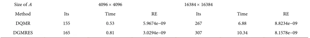
Method Its Time RE Its Time RE DQMR 155 0.53 5.9674e−09 267 6.88 8.8234e−09 DGMRES 165 0.81 3.0294e−09 307 10.34 8.1578e−09
required for convergence, the relative error (RE), for the DGMRES and DQMR methods. As shown in Table 1, Table 2 the DQMR algorithm is effective and less expensive than the DGMRES algorithm.
5. Conclusion
In this paper, we presented a new method, called DQMR, for Drazin-inverse solution of singular nonsymmetric linear systems. The DQMR algorithm for singular systems is analogous to the QMR algorithm for non-singular systems. Numerical experiments indi- cate that the Drazin-inverse solution obtained by this method is reasonably accurate, and its computation time is less than that of solution obtained by the DGMRES method. Thus, we can conclude that the DQMR algorithm is a robust and efficient tool to com- pute the Drazin-inverse solution of singular linear systems.
Acknowledgements
First, we would like to thank professor F. Toutounian for her comments that improved our results. Second, we thank the editor and the referees for their carefully reading and useful comments.
References
[1] Ben-Israel, A. and Grevile, T.N.E. (2003) Generalized Inverses: Theory and Applications. 2nd Edition, Springer-Verlag, New York.
[2] Campell, S.L. and Meyer, C.D. (1979) Generalized Inverses of Linear Transformations. Pitman (Advanced Publishing Program), Boston.
[3] Hartwig, R.E. and Hall, F. (1982) Applications of the Drazin Inverse to Cesaro-Neumann Iterations. In: Campbell, S.L., Ed., Recent Applications of Generalized Inverses, 66, 145-195. [4] Hartwig, R.E. and Levine, J. (1981) Applications of the Drazin Inverse to the Hill Crypto-
graphic system. Part III, Cryptologia, 5, 67-77. https://doi.org/10.1080/0161-118191855850
[image:11.595.41.556.187.250.2][6] Freund, R.W. and Hochbruck, M. (1994) On the Use of Two QMR Algorithms for Solving Singular Systems and Applications in Markov Chain Modeling. Numerical Linear Algebra with Applications, 1, 403-420. https://doi.org/10.1002/nla.1680010406
[7] Simeon, B., Fuhrer, C. and Rentrop, P. (1993) The Drazin Inverse in Multibody System Dynamics. Numerische Mathematik, 64, 521-539. https://doi.org/10.1007/BF01388703
[8] Brown, P.N. and Walker, H.F. (1997) GMRES on (Nearly) Singular Systems. SIAM Journal on Matrix Analysis and Applications, 18, 37-51.
https://doi.org/10.1137/S0895479894262339
[9] Ipsen, I.F. and Meyer, C.D. (1998) The Idea behind Krylov Methods. The American Ma-thematical Monthly, 105, 889-899. https://doi.org/10.2307/2589281
[10] Smoch, L. (1999) Some Result about GMRES in the Singular Case. Numerical Algorithms, 22, 193-212. https://doi.org/10.1023/A:1019162908926
[11] Wei, Y. and Wu, H. (2000) Convergence Properties of Krylov Subspace Methods for Singu-lar System with Arbitrary Index. Journal of Computational and Applied Mathematics, 114, 305-318. https://doi.org/10.1016/S0377-0427(99)90237-6
[12] Sidi, A. (1999) A Unified Approach to Krylov Subspace Methods for the Drazin-Inverse Solution of Singular Non-Symmetric Linear Systems. Linear Algebra and Its Applications, 298, 99-113. https://doi.org/10.1016/S0024-3795(99)00153-6
[13] Sidi, A. and Kluzner, V. (1999) A Bi-CG Type Iterative Method for Drazin Inverse Solution of Singular Inconsistent Non-Symmetric Linear Systems of Arbitrary Index. The Electronic Journal of Linear Algebra, 6, 72-94.
[14] Sidi, A. (2001) DGMRES: A GMRES-Type Algorithm for Drazin-Inverse Solution of Sin-gular Non-Symmetric Linear Systems. Linear Algebra and Its Applications, 335, 189-204.
https://doi.org/10.1016/S0024-3795(01)00289-0
[15] Zhou, J. and Wei, Y. (2004) DFOM Algorithm and Error Analysis for Projection Methods for Solving Singular Linear System. Applied Mathematics and Computation, 157, 313-329.
https://doi.org/10.1016/j.amc.2003.08.036
[16] Lanczos, C. (1950) An Iteration Method for the Solution of the Eigenvalue Problem of Li-near Differential and Integral Operators. Journal of Research of the National Bureau of Standards, 45, 255-282. https://doi.org/10.6028/jres.045.026
[17] Saad, Y. (2003) Iterative Methods for Sparse Linear Systems. 2nd Edition, SIAM, Philadel-phia. https://doi.org/10.1137/1.9780898718003
Submit or recommend next manuscript to SCIRP and we will provide best service for you:
Accepting pre-submission inquiries through Email, Facebook, LinkedIn, Twitter, etc. A wide selection of journals (inclusive of 9 subjects, more than 200 journals)
Providing 24-hour high-quality service User-friendly online submission system Fair and swift peer-review system
Efficient typesetting and proofreading procedure
Display of the result of downloads and visits, as well as the number of cited articles Maximum dissemination of your research work