Munich Personal RePEc Archive
Intergenerational complementarities in
education, endogenous public policy, and
the relation between growth and
volatility
Palivos, Theodore and Varvarigos, Dimitrios
University of Macedonia, University of Leicester
16 April 2011
Online at
https://mpra.ub.uni-muenchen.de/31343/
Intergenerational Complementarities in Education, Endogenous
Public Policy, and the Relation between Growth and Volatility
Theodore Palivos
aDimitrios
Varvarigos
bUniversity of Macedonia, Greece
University of Leicester, UK
Abstract
We construct an overlapping generations model in which parents vote on the tax rate that determines publicly provided education and offspring choose their effort in learning activities. The technology governing the accumulation of human capital allows these decisions to be strategic complements. In the presence of coordination failure, indeterminacy and, possibly, growth volatility emerge. This indeterminacy can be eliminated by an institutional mechanism that commits to a minimum level of public education provision. Given that, in the latter case, the economy moves along a uniquely determined balanced growth path, we argue that such structural differences can account for the negative correlation between volatility and growth.
Keywords: Human Capital, Economic Growth, Endogenous Taxation, Volatility
JEL Classification: H42, H52, O41.
a Address: Department of Economics, 156 Egnatia Street, Thessalonica GR-540 06, Greece. Email:
[email protected]. Tel: +30 2310 891 755
b Address: Department of Economics, Astley Clarke Building, University Road, Leicester LE1 7RH, UK.
1 Introduction
Investment in formal education is one of the most important intergenerational transfers. It is
considered as a key factor of economic growth and income distribution. Several aspects of
this investment have been analysed in the literature. For example, Glomm and Ravikumar
(1992) examine the effects of public and private education on long-run growth and
inequality. Bénabou (1996) considers how the growth performance of an economy is
influenced by the degree of decentralization of government funding for education.
Blankenau and Simpson (2004) show conditions under which the effect of public education
spending on growth may be non-monotonic. Cremer and Pestieau (2006) study the design of
optimal education policy. Finally, Kempf and Moizeau (2009) investigate the link between
social segmentation, inequality and growth in an environment where education is a club
good.
This paper complements the existing literature by highlighting the fact that, unlike the
production of physical capital, the education process involves the decisions of two
consecutive generations, parents and children. The first generation, parents/tax payers,
provides the resources for education (e.g., teachers’ salaries, buildings, equipment, etc.) and
the second, children/students, the time and effort that are necessary to absorb knowledge.
Moreover, insofar as the actions by one generation affect the outcome for the other, one of
the important characteristics that may affect each generation’s decisions and actions is its
reflection of how the other will decide and act. Put differently, the education process entails
the coordination of the decisions made by two generations, which may be strategic
complements (see, Cooper and John 1988).1
The idea that there may be a coordination game inherent in the accumulation of human
capital seems particularly relevant in the case of public education, where decisions are often
made collectively by a large number of individuals through voting. More specifically, the
voters’ support towards public investment for education may depend on the extent to which
the younger generation will provide the learning effort necessary for allowing them to ‘reap’
the benefits associated with more widely spread and qualitatively improved education
services. Nevertheless, the return to the young generation’s learning effort may be partially
1 Strategic complementarity “implies that an increase in the action of all agents except agent i increases the
determined by the qualitative characteristics of the education sector – characteristics that
depend on public investment. One expects that such cross-generational interactions will
have important repercussions for human capital accumulation and, consequently, economic
growth. Nevertheless, the aforementioned literature on public education and growth has
largely neglected the strategic complementarities that are inherent to decisions of coexisting
cohorts of agents with different objectives – decisions which jointly determine the formation
of human capital.
Our analysis builds upon an overlapping generations model in which the engine of
growth is the accumulation of human capital. The actions of both young (offspring) and
adults (parents) affect the formation of human capital. In particular, the parents vote on the
tax rate that determines the revenue available to the government for the provision of public
education, while the offspring decide on the effort they devote towards learning activities.
The technology governing the evolution of human capital allows these decisions to be
strategic complements. Specifically, in equilibrium, the effort devoted by the young is an
increasing function of the tax rate chosen by parents which, by itself, is an increasing
function of the offspring’s learning effort.
First, we show that a coordination failure may arise and multiple equilibria emerge. These
equilibria are Pareto-ranked. They include an equilibrium in which both cohorts choose no
provision (i.e., no effort by offspring and a zero tax rate chosen by parents), and equilibria
entailing positive effort by the young and a positive tax rate by the adult voters. Thus, as in
Redding (1996) and Palivos (2001) among others, our paper provides an explanation for the
persistent disparities in the world distribution of incomes and growth rates, which differs
from the “path dependence” hypothesis – a hypothesis that has been criticized on the basis
that many industrialized countries did not happen to be rich at the initial stages of their
development and yet the managed to cross the threshold level. 2 Why is it that currently poor
countries cannot cross it?
Naturally, the idea that multiple growth paths may be attributed to failures of
coordination offers support for some type of government intervention (be it in terms of
economic policy or a more structural/institutional reform) that is designed to induce the
2 Examples of path-dependent multiple equilibria are provided in the analyses of Azariadis and Drazen (1990),
selection of the economically/socially “preferable” equilibrium. For this reason, we
subsequently consider an institutional reform that could induce the selection of the “high
growth/high welfare” equilibrium. In particular, we show that the commitment to a
sufficiently high tax can achieve this objective and, therefore, eliminate growth
indeterminacy.
In addition to the above, we are able to show that one of the most pervasive empirical
regularities in macroeconomic data, the negative relation between output growth and its
volatility, can be attributed to the intergenerational complementarities as well as to the public
sector’s institutional arrangements.3 The explanation we offer works as follows. The
existence of multiple growth equilibria possesses an additional explanatory power when it
comes to the overall macroeconomic performance. In a dynamic setting, there is nothing to
preclude the possibility that in some periods agents may choose actions associated with high
growth while in other periods they may choose actions associated with low growth. Periods
of strong economic activity may be followed by periods of weak economic activity and vice
versa, depending on how some agents expect others to behave and act. Thus, growth
indeterminacy is inherently linked with the idea of growth volatility. We show that the
average growth rate in this case is lower compared to the uniquely determined growth rate
that emerges in the presence of a minimum commitment to public education.
By providing an alternative suggestion, our analysis may be viewed as complementary to a
series of theoretical papers that employ stochastic growth models in order to examine the
impact of public policy on the growth-volatility nexus (e.g., Turnovsky, 2000; Blackburn and
Pelloni, 2004; Chatterjee et al., 2004; Varvarigos, 2007). In these models, exogenous variations
in policy parameters cause changes in both the average growth rate and its volatility. In
contrast, we attribute this relation to the structural characteristics pertaining to the endogenous
determination of public policy.
The implications from our model share some similarities with those in the interesting and
important, but largely neglected, paper of Glomm and Ravikumar (1995). They also show
that the presence of endogenously determined public spending may generate, rather than
eliminate, equilibrium indeterminacy, sending thus a cautionary message regarding the role of
public policy. Nevertheless, there are also significant differences between their analysis and
3 Evidence on the negative relation between output growth and its volatility is provided by Turnovsky and
ours. Firstly, they do not examine the relation between growth and volatility as we do in this
paper. Secondly, the mechanism leading to their result is different as it rests on the ideas
that, (i) the young generation’s education effort depends on the expectation of the future tax
rate that will be chosen by the same generation when it becomes old, and (ii) the chosen tax
rate depends on aggregate human capital due to the fact that the ‘warm glow’ argument in
the utility function is introduced with CRRA coefficient which is different in comparison to
the one attached to the remaining utility arguments; therefore, their result is not due to
strategic complementarities in the decision making process of two distinct cohorts of agents.
Put differently, we find multiple equilibria even with simple functional forms that imply
uniqueness in their model. Moreover, equilibria cannot be Pareto ranked in their model,
whereas, in our case, the high-growth equilibrium yields higher welfare. Finally, when their
parameter values allow multiple equilibria, they find an inverse relation between the tax rate
and income. In contrast, our model shows that the high-growth equilibrium actually
corresponds to the relatively high tax rate.
Although this last result appears to be in contrast to conventional wisdom, it is not
completely at odds with existing empirical evidence, especially when considering the
productive use of tax receipts in our model. While many analyses are unable to derive a
decisive conclusion on the growth effects of taxation and public spending – see Myles
(2000), Agell et al. (2006) and Bania et al. (2007) for example – when econometric methods
account for the productive use of public spending (infrastructure investment, education etc.)
then there is supportive evidence of positive effects from taxation/public spending to
economic growth (e.g., Mofidi and Stone, 1990; Pereira, 1998; Kneller et al., 1998; Cohen and
Paul, 2004). In fact, in his survey of the relevant literature, Poot (2000) claims that “the most
conclusive results in the literature relate to the positive impact of education expenditures on
growth” (Poot, 2000; p. 516) – thus, providing further support on this element of our
results.
The rest of the paper is structured as follows. Section 2 presents the general set-up of the
model. Section 3 establishes the existence of multiple equilibria and analyzes its implications.
Section 4 shows that growth indeterminacy can be eliminated with partial commitment on
behalf of the government. Section 5 examines the same issue under alternative arrangements
2 The Basic Structure
We consider an overlapping generations economy in which time is discrete and indexed by
0,1, 2...
t = . Each period, a cohort of unit mass is born. Agents within the cohort are
identical and live for two periods. They are ‘young’ (or ‘offspring’) in the first period of their
lifetime and ‘old adults’ (or ‘parents’) in the second. All agents are endowed with one unit of
time in each period. The young allocate it between activities that augment their human
capital (e.g., formal schooling) and leisure. The old, on other hand, supply their time,
combined with their human capital (determining knowledge, efficiency and expertise),
inelastically to firms in exchange for the prevailing market wage. Adults are also ‘voters’ in
the sense that they cast a vote on their preferred tax rate that the government imposes on
their labour income. Their disposable income (i.e., the residual after taxation) finances their
consumption. The revenues collected by the government are utilised so as to finance
activities that support the qualitative characteristics of education (e.g., the quality of
schools/colleges/universities, scholarships, research and teaching support etc.) and,
therefore, promote the formation of human capital. The government abides by a
balanced-budget rule each period.
An agent born in period t enjoys utility over her whole lifetime according to4
1 2 2
ln(1 ) ln( ) ln( )
t
t t t t
u = −e + c+ + w +h+ , (1)
where et denotes schooling effort when young and ct+1 denotes consumption when old. 5 We
implicitly assume that children’s consumption is incorporated into the consumption of
parents. The last term of the utility function indicates that parents are imperfectly altruistic
towards their offspring. Specifically, a parent gets satisfaction from her offspring’s realised
income. This is meant to capture the idea that parents care about their offspring’s future
prospects and social status (both being enhanced through more advanced knowledge and/or
increased income).
We assume that, when young, a person can pick up a fraction v∈(0,1) of the existing
(average) level of human capital Ht without effort. This may happen, for example, through
4 We choose equal weights in the utility function purely for simplicity. The more general case is analysed in
Palivos and Varvarigos (2009).
5 The superscript t on the left-hand side indicates the time of birth of the generation enjoying utility through
some type of home tutoring or by simple observation. The government provides goods and
services that increase the potential human capital that a young person can acquire even
further. Nevertheless, the young person must provide resources that take the form of effort
(or foregone leisure), denoted by et, in order to benefit from the government’s offer of
education. Specifically, the formation of human capital takes place according to the learning
technology6
1
t t t t
h+ =vH +φg e , (2)
where gt denotes public expenditure per student and the parameter φ>0 captures the
efficiency of the public education system.7
All adults are liable to income taxation. Therefore, they will meet their consumption
needs out of their disposable income. Thus, the budget constraint during adulthood is
1 (1 1) 1 1
t t t t
c + = −τ + w h+ + . (3)
The government finances the provision of goods and services towards education by
utilising its total revenue from labour income taxation τtw Ht t. Given that there is a unit
mass of young agents and the population size remains constant, spending per student
corresponds to
t t t t
g =τ w H . (4)
The single and perishable consumption good that exists in this economy is produced and
supplied by perfectly competitive firms, who employ efficient labour so as to produce Yt
units of output according to
t t
Y =AH , A>0. (5)
Notice that besides the level of human capital, Ht also corresponds to the economy’s
available units of efficient labour, because adult agents (whose large population is normalised
6 This technology for the accumulation of human capital shares common features with de Gregorio and Kim
(2000) and Ceroni (2001) among others. However, none of these have combined both effort (by offspring) and endogenously determined resources (by voters and the public sector) as complementary inputs within the same type of technology. Glomm and Ravikumar (1992, 1995) include both types of inputs in the formation of human capital, but they also assume that each input is essential for a positive stock of human capital.
7 We assume a linear effect for t
to one) supply one unit of ‘raw’ time each. Profit maximisation implies that the equilibrium
market wage per unit of (efficient) labour is wt =A ∀t.
As indicated earlier, the electorate is comprised by the adults who cast a vote on their
preferred tax rate. Therefore, the problem of an agent born it t is to choose et, ct+1 and τt+1
so as to maximise (1) subject to (2), (3), (4), 0≤ ≤et 1, 0≤τt+1≤1, and ct+1≥0, taking Ht,
1
t
H+ , wt, wt+1 and wt+2 as given. Of course, given that individuals are identical, the tax rate
chosen by the representative parent is the one that will prevail in a democratic regime.
Equivalently, we can substitute (2)-(4) in (1) and write lifetime utility as
1 1 2 1 1 1 1 1
ln(1 ) ln[(1 ) ( )] ln[ ( )]
t
t t t t t t t t t t t t t t
u = −e + −τ + w+ vH +φeτ w H + w+ vH+ +φe+τ +w H+ + . (6)
It is straightforward to check that the FOC associated with the problem of an individual
who was born in period t can be eventually written as
1
, 0 1
t t t
t
t t t t t t
φτ w H
e e ≥vH φτ w H e ≥
− + , (7)
and
1 1 1
1 1 1 1 1 1 1
1
, 0
1
t t t
t
t t t t t t
φw H e τ
τ vH φτ w H e
+ + +
+
+ + + + + +
≥ ≥
− + , (8)
with complementary slackness in both (7) and (8). Notice that we can use (8) to infer the tax
rate that will be chosen by adults who were born in period t−1 (that is, the parents of
agents born in period t).
3 Equilibrium Analysis
In this section we establish the existence of multiple equilibria and analyse their implications
for macroeconomic outcomes as well as for institutional arrangements pertaining to public
policy.
3.1 Multiplicity of Equilibria
We can view the situation described here as a game played between each pair of consecutive
generations, that is, between parents and children. Each agent plays this game twice, once as
chooses the amount of resources that will be allocated to public education by casting a vote
on the preferred tax rate τt. At the same time, the child chooses the amount of her time, or
equivalently her effort, et, that she will devote on schooling. Nevertheless, when deciding
her choice variable, each player takes the action of the other player as given. If we substitute
the equilibrium conditions ht =Ht and wt =A in equations (7) and (8), both dated in
period t, and take into account the constraints 0≤ ≤et 1and 0≤ ≤τt 1, we can derive the
best response function of each generation, that is,
1
max 0, 1
2 t t γ e τ ⎧ ⎛ ⎞⎫ ⎪ ⎪ = ⎨ ⎜ − ⎟⎬ ⎪ ⎝ ⎠⎪
⎩ ⎭, (9)
and
1
max 0, 1
2 t t γ τ e ⎧ ⎛ ⎞⎫ ⎪ ⎪ = ⎨ ⎜ − ⎟⎬ ⎪ ⎝ ⎠⎪
⎩ ⎭, (10)
where γ=v/φA. The equilibrium values of τt and et are given by the intersection of (9)
and (10). Given that ,τt et∈[0,1], we can summarise these solutions as
0 if 0 otherwise t t τ γ e > > ⎧ ⎪ ⎨ ⎪= ⎩
, and
0 if 0 otherwise t t e γ τ > > ⎧ ⎪ ⎨ ⎪ = ⎩ . (11)
These results merit some discussion. First of all, we see that corner solutions are possible
and, as a result, et = =τt 0 is an equilibrium. Evidently, this is due to the effect of the
composite term γ which stems, mainly, from the presence of the parameter v. The intuition
is that, as long as v>0, the marginal utility has a finite upper bound for zero values of et or
t
τ . Therefore, such choices are possible due to the fact that utility may become
monotonically decreasing in these arguments. Secondly, as indicated in (11), children will
devote a positive level of effort or time in schooling only if they expect a minimum level of
resources allocated to public education. Moreover, if positive, the effort on schooling
depends negatively on v, the fraction of human capital transferred to the next generation
without any effort, and positively on the efficiency of the schooling system (φ) and the wage
rate (A)(see equation 9). Thirdly, parents behave analogously (see equations 10 and 11). In
allocate a positive fraction of the existing resources on public education. This fraction, if
positive, depends also negatively on v and positively on φ and A.
As indicated above, additional interior solutions with both et and τt being positive are
possible as well, meaning that the model may actually admit multiple equilibria. The
underlying cause of multiple equilibria in this framework is the strategic complementarity
between the decisions of the two groups, which mutually reinforce one another (see Cooper
and John, 1988). More specifically, as it can be seen form equations (9) and (10), a higher
activity by one cohort of agents induces the other cohort to increase its activity as well. Once
more, the presence of the parameter v (which implies a positive γ) is responsible for these
effects. We can clearly see that when v =0 (γ=0), both solutions become invariant to each
other. The intuition is that, for v =0, the marginal utilities of both et and τt depend only on
the relative weights of the utility arguments that they ultimately affect (in this case, the
arguments are equally weighted). When v>0, however, the marginal utility of et (τt) is
increasing in τt (et). Following increases in these variables, individuals will restore the
equilibrium by taking the appropriate action so as to reduce their marginal utility –
something they can do with an increase in et (τt) . In terms of intuition, a higher tax rate
implies an increase in publicly provided education, therefore an increase in the benefits from
devoting effort towards human capital accumulation. Similarly, a greater education effort by
the young increases their parents’ marginal utility benefit of foregoing consumption and
choosing a higher tax rate, a benefit that is due to the presence of the ‘warm-glow’ element
in their preferences.
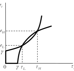
Figure 1. Multiple equilibria
t
e
t
τ
0 γ
γ
L
τ τH
L
e
H
[image:11.595.229.381.551.697.2]The situation described above is depicted in Figure 1. We can describe it, more formally,
in
Proposition 1. There exist at most three pure strategy equilibria. These are {0, 0}, { ,eL τL} and
{ ,eH τH} where,
1 1 8
4
1 1 8
4
L
t
H
γ
e
e
γ
e
⎧ − −
= ⎪ ⎪⎪ = ⎨
⎪ + −
⎪ = ⎪⎩
. (12)
and
L L
t
H H
τ e
τ
τ e
= ⎧ ⎪ = ⎨
⎪ =
⎩
. (13)
Proof: All proofs are relegated to the Appendix.
As long as γ<1/ 8 (henceforth, a condition that we assume to hold) the results in (12)
and (13) show that it is possible to get interior equilibria in addition to the corner solution.8
The next step of our analysis is to examine whether the multiplicity of equilibria rests upon
the presence of a coordination failure in the decision making process by the young and the
old. In contrast to Glomm and Ravikumar (1995) and Palivos (2001), whose frameworks
involve trade-offs that do not allow, in general, the Pareto ranking of equilibria, we can
establish such ranking through
Lemma 1.The three equilibria are ranked in the Pareto sense.
To complete the characterisation of the different equilibria, we need to address the issue
of their stability. In other words, we need to consider whether small perturbations in the
8 The equality between the equilibrium values of t
neighbourhood of each set of equilibrium choices will leave these choices unaffected or not.
As it is known from the analysis of Cooper and John (1988), not all possible equilibria of a
coordination game are unresponsive to such perturbations, as one of them may be locally
unstable. In our model, such an equilibrium is represented by the point { ,eL τL}. This
becomes evident from the fact that ∂eL /∂ >γ 0 and ∂τL/∂ >γ 0 – results that are
completely at odds with the nature of the best-response functions in (9) and (10). If
anything, we would expect that both cohorts choose lower values when the composite
parameter term γ is higher, as they actually do at { ,eH τH}. Thus, the point { ,eL τL}
represents nothing else but a threshold which, in conjunction with agents’ expectations of
how others will act, determines which of the two stable equilibria – i.e., {0, 0} or { ,eH τH} –
will prevail. For example, consider that each cohort makes a choice x, where x =e,τ. If one
cohort expects the other to choose x<xL (x >xL), then it will choose 0 (xH).
Anticipating this, the other cohort will choose 0<xL (xH >xL), thus verifying the initial
expectation. 9
3.2 Further Implications
As we have seen, when decisions by the young and the old within a given period are strategic
complements, and in the presence of a coordination failure, the model can generate multiple
equilibria. Moreover, what is particularly interesting with our analysis is the idea of output
growth indeterminacy that arises because any of the two equilibria can prevail: for a given
t
H , next period’s human capital (which, in equilibrium, satisfies ht+1=Ht+1) can take more
than one possible values. The indeterminacy of equlibria, which, as argued intuitively above
and shown formally in Sections 4 and 5 below, emerges because of the endogenous determination
of public policy, has the following two additional implications.
Firstly, it results in indeterminacy of the growth rate of output and human capital, since
1/ 1/ .
t t t t t t
Y+ Y =H + H = +v ωeτ Thus, our paper belongs to the strand of literature that
9 Notice that this notion of instability differs from the one applied in variables that display an explicit dynamic
pattern. More formally, let et = f( )τt and τt =Φ( )et denote the best-response function of the children and the
illustrates the stylised fact of ‘club’ convergence, without resorting to the problematic
scenario in which growth/development paths depend on initial conditions or endowments –
problematic in the sense that the suggestion that some countries are currently rich simply
because they happened to be rich before does not appear to be historically accurate. Other
analyses that arrive to similar conclusions, but under different settings, are those of Redding
(1996) and Palivos (2001). In the former, strategic complementarities between workers and
entrepreneurs imply that, over some range of parameter values, multiple growth equilibria
may emerge. In the latter, the complementarities generated by the existence of family-size
norms imply indeterminate fertility choices and, given the trade-off between child-rearing
and educational attainment, multiple growth equilibria.
The second significant implication of indeterminacy is that the growth rate of output may
not settle down to a balanced growth path, instead its behaviour may display a periodic
pattern. In fact, any of the two equilibria
{ }
0, 0 and{
eH,τH}
may prevail during eachdistinct period t∈ ∞[0, ).10 We can formalise this argument with
Proposition 2. The growth rate of output may not be balanced, instead it may be volatile as it is given by
1 1
ˆt ( , )ˆ ˆt t t / t t / t ˆ ˆt t
η η≡ e τ =Y+ Y =H+ H = +v ωeτ , where { , } {0, 0} eˆ ˆt τt = or { , } { ,eˆ ˆt τt = eH τH}, for
any t ≥0.
The idea of volatile growth is absent from the analysis of Redding (1996) because he
employs a framework in which the economy terminates at the end of the second period,
implying that interactions among agents occur only once: consequently, multiple equilibria
cannot be considered as a sign of periodic fluctuations in economic activity. In this respect,
our framework shares more similarities with the analysis of Palivos (2001) in the sense that
both employ full-fledged dynamic settings which allow interactions between agents to occur
10 An important feature that leads to the emergence of multiple equilibria is the assumption that individuals
decide optimally on how much time or effort they devote towards learning activities. Some may argue that the introduction of compulsory schooling may invalidate this idea, in which case multiple equilibria (and growth volatility) disappear. However, there are strong arguments against this conjecture. First, even if attendance to some basic education (schooling) is mandatory, there are always elements in the education system that are not compulsory (e.g., higher education). Second, even if someone interprets et in the narrow sense of ‘schooling’
at every distinct period. Like we do in this paper, he recognises that multiplicity and
indeterminacy are sources of growth volatility. In a framework which is closer to ours,
Glomm and Ravikumar (1995) also discuss the possibility of cycles due to the presence of
multiple equilibria. In their model, these arise (under some parameter specifications) because
the future tax rate, which depends on future income, affects current education decisions
which, partially, determine future income due to the accumulation of human capital.
Notwithstanding these common equilibrium implications, our particular framework
offers new dimensions in two different respects: firstly, in the type of interactions that
generate these effects and, secondly, in the implications for public policy. The latter issue is
particularly pertinent, that is why we discuss it and analyse it formally in the subsequent part
of our paper.
4 Equilibrium with Partial Commitment
Given that the equilibria are Pareto-ranked, there is a clear scope for government
intervention that will induce the selection of the “high growth/high welfare” equilibrium,
represented by the pair
{
eH,τH}
. Nevertheless, the preceding analysis has shown that theunderlying source of indeterminacy and, therefore, growth volatility is inherently linked to
the endogenous determination of public policy itself. For this reason, it may be instructive to
seek a more institutional-oriented arrangement that could act as the desired selection
mechanism.
As it will transpire from the following analysis, such an institutional mechanism exists.
Suppose that, irrespective of the choices made by voters (which may approximate the
ideological stance of different political parties), the government commits a minimum
fraction (0,1)s∈ of the economy’s output for public education expenditures. Given the
other assumptions of the model, s is also the minimum tax rate that adults will pay
irrespective of their choices. However, they may choose to vote for a tax rate which is higher
than s. Denoting this incremental tax (i.e., the increment over s) that adults may vote for by
t
q , and given that the total amount of tax revenues supports public expenditures towards
the formation of human capital, the lifetime utility function is now given by
1 1
2 1 1 1 1 1
ln(1 ) ln{(1 ) [ ( ) ]}
ln{ [ ( ) ]}.
t
t t t t t t t t
t t t t t t
u e s q w vH φe s q w H
w vH φe s q w H
+ +
+ + + + + +
= − + − − + +
It should be noted here that a scenario in which governments commit to the provision of
a certain fraction of GDP or of tax revenue towards education spending is not just a
theoretical construction; instead there are instances where such mechanisms have been
actually implemented. For example, Section 8 of Article XVI of the California state
constitution, added by Proposition 98 of 1988, establishes a minimum funding level or
guarantee for K–12 education and community colleges (Leyden, 2005).
Now, the lifetime utility in (6) is replaced by the one in (14). Following the same steps as
before, it is straightforward to establish that the best response functions are given by
1
max 0, 1
2 t t γ e s q ⎧ ⎛ ⎞⎫ ⎪ ⎪ = ⎨ ⎜ − ⎟⎬ + ⎪ ⎝ ⎠⎪
⎩ ⎭, (15)
and
1
max 0, 1 2
2 t t γ q s e ⎧ ⎛ ⎞⎫ ⎪ ⎪ = ⎨ ⎜ − − ⎟⎬ ⎪ ⎝ ⎠⎪
⎩ ⎭. (16)
Solving (15) and (16) simultaneously, we find that et is the same as the one given by (12),
while
L L
t
H H
q τ s q
q τ s
= − ⎧ ⎪ = ⎨ ⎪ = − ⎩ , (17)
where, τL and τH are given in (13). Thus, the results in (12) and (17) allow us to derive
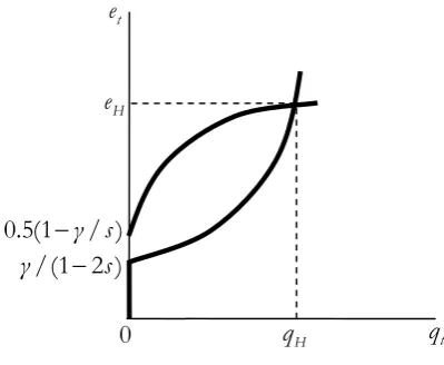
Proposition 3. As long as s∈
(
τ τL, H)
, there exists a unique equilibrium { ,eH qH}. Consequently,the growth rate of the economy is balanced and equal to η η≡ ( , )eˆ ˆt τt =Yt+1/Y =Ht+1/Ht
( ).
H H
v ωe s q
= + + Furthermore, it is s+qH =τH.
The preceding analysis shows that an institutional arrangement that commits a sufficient
fraction of output towards public education can act as an efficient mechanism that will
induce the coordination towards a unique equilibrium. In particular, the equilibrium selected
will replicate the “high growth/high welfare” equilibrium which we derived in a preceding
This result is quite intuitive. A sufficiently high s will induce the young to choose a
relatively high effort towards learning activities. The adult voters recognise this and respond
optimally by choosing a positive increment over the minimum tax rate s. This choice
induces even higher levels of learning effort by the young. Thus, it verifies the adults’
expectations that induced them to support public education through a sufficiently high
overall tax rate.
Figure 2. Unique equilibrium
4.1 Public Education Spending and the Relation between Growth and
Volatility
Due to its ability to induce the selection of the “high growth/high welfare” equilibrium, the
commitment to a sufficiently high share of public education can also eliminate growth
volatility. Therefore, the structural characteristics pertaining to the endogenous
determination of public spending on education may allow us to derive a novel explanation
for one of the most pervasive macroeconomic facts, i.e., the relation between output growth
and its volatility.
Despite the fact that some early economists conjectured that temporary and long-term
movements in economic activity are inherently linked, it is only recently that a growing body
of literature considered the analysis of the fundamentals behind this link as a research
question worth pursuing. This strand of literature was further stimulated by an increasing
number of empirical analyses (see footnote 3) showing that growth rates are significantly –
and, mainly, inversely – correlated, on average, with proxies of their variability. Until
recently, theoretical studies have explored this issue with the construction and solution of
t
e
t
q
0 /(1 2 )
γ − s
H
q
0.5(1−γ/ )s
H
[image:17.595.165.365.229.393.2]stochastic endogenous growth models – i.e., models in which (extrinsic) uncertainty is
introduced through the incorporation of some RBC-type real and/or monetary shocks in
frameworks that endogenise the process of productivity improvements. As a result, in
models such as those of Turnovsky (2000), Blackburn and Pelloni (2004), Chatterjee et al.,
(2004) and Varvarigos (2007), the decisions governing the formation of the reproducible
factor of production (be it physical or human capital) respond optimally to the realisation of
stochastic shocks, therefore the average growth rate is affected by the volatility of these
shocks. Using such frameworks, the authors have examined how exogenous variations in policy
parameters affect both the average growth rate and its volatility.
Our analysis can be viewed as providing an alternative suggestion – mainly, the idea that
both differences in growth rates and the incidence of growth volatility are inherently linked
to the structural characteristics of endogenously determined economic policy. On the one hand,
growth volatility is an outcome related to the manner through which public policy is
endogenously determined; on the other hand, such volatility may be eradicated by an
institutional mechanism that commits some fraction of the economy’s output towards public
education spending. We outline the main implication from this idea in
Proposition 4. There is a negative correlation between volatility and growth, in the sense that the average
growth rate of the economy that may undergo fluctuations is lower than the average growth rate of the economy
in which a minimum commitment eliminates these fluctuations. That is, E( )ηˆt <E( )η
.
Contrary to the existing literature, our model does not rely on exogenously introduced
random shocks so as to generate growth volatility. Rather, it is the intrinsic uncertainty that
is inherent in strategically complement decisions, when these are subjected to coordination
failure, which is responsible for growth volatility.11 When the structural characteristics of the
economy render such failures absent, variability disappears and the complementary actions
by agents are conducive to the formation of human capital. Given that elements of public
11 A recent contribution by Wang and Wen (2006) also examines the relation between endogenously driven
policy are embedded to these structural characteristics, our framework suggests that a
macroeconomic phenomenon – that is, the correlation between output growth and its
volatility – may be attributed to issues pertaining to the field of public economics.
What needs to be stressed at this point is that although we provide an alternative
explanation to that of the aforementioned analyses of stochastic endogenous growth, we do
not view these different suggestions as being mutually exclusive. Rather, we view our result
as complementary to existing ones given that nothing precludes the possibility that the
relation between growth and volatility nests factors that relate to both exogenous shocks and
failures of coordination. So far, the existing empirical literature has not provided a definite
answer on which type of framework is more appropriate in identifying the underlying forces
that govern the relation between economic growth and macroeconomic volatility. However,
existing empirical studies have actually shown that models including coordination failures
can be successful in capturing pervasive stylised facts of actual business cycles – see for
example, Cooper and Haltiwanger (1996). Such evidence provides definite support for our
result’s validity in suggesting a complementary explanation for the existence of a relation
between volatility and output growth.
5 Outcomes with Full Commitment
So far, our formal analysis has been based on a scenario where choices by both the young
and the old are formed through some type of coordination game. In this Section, we will
reconsider these interactions under an alternative set-up. In particular, we will examine cases
in which one of the two cohorts acts as a Stackelberg leader in the game that determines the
optimal choices.
5.1 The Adult Voters as Leaders
We shall assume that the old decide on the tax rate first and, following this announcement,
the young decide on their education effort. Effectively, this scenario is conceptually similar
to the one described in Section 4. In particular, the government (through the voting
behaviour of the old) commits to the level of public education spending reflected in the
More specifically, this approach entails that we solve the problem of a young person in
period t so as to get her best-response function et = f( )τt . The old adults of generation
1
t − will take account of this when choosing their preferred tax, τt; therefore, the effort
level chosen by the young will be et = f( )τt . Maximising (1) with respect to et yields
1 1
t t t
t t t t t t
φτ w H
e =vH φτ w H e
− + . (18)
Solving (18) for et gives
1 1 2 t t t v e φτ w ⎛ ⎞ = ⎜ − ⎟
⎝ ⎠. (19)
Our next step is to substitute (19) into the t−1 variant of the utility function given in (1).
Eventually, we get
1
1 1 1 1 1 1
ln(1 ) ln[(1 ) ( )] ln ( )
2
t
t t t t t t t t t t t t
w
e− τ w vH− φτ −w H e− − − ⎡ + vH φτw H ⎤
− + − + + ⎢ + ⎥
⎣ ⎦. (20)
Maximising (20) with respect to τt yields
1 1
t t
t t t t t
φw H
τ =vH φτ w H
− + . (21)
Now, we can substitute wt =A and γ=v/φA in (21), and solve for τt to get
1 2
t
γ
τ = − ≡τ. (22)
Finally, substituting (22) in (19) gives us
1 1 3 2 1 t γ e e γ ⎛ − ⎞ = ⎜ ⎟≡ −
⎝ ⎠ . (23)
As long as the previously imposed restriction γ<1/ 8 still applies (which we assume it
does), these solutions satisfy γ τ< < 1 and γ< <e 1 as required. Thus, we can present our next result in the form of
Proposition 5.The equilibrium growth rate is equal to η≡Yt+1/Yt =Ht+1/Ht = +v ωτe, for every
0
It is evident that, in this scenario, the equilibrium is unique and the possibility of growth
variability has disappeared. In terms of intuition, the intrinsic uncertainty that pertained
choices when these were made through a coordination game has vanished. The old
understand that an increase in the tax rate increases the willingness of the young to forego
part of their leisure activities, simply because the benefits from doing so are higher.
Consequently, they decide the tax rate that will induce children to provide the relatively high
education effort that will satisfy their parents.
5.2 The Young as Leaders
Although it represents a less reasonable scenario, we shall briefly discuss the case where the
young are the ones who commit to a certain effort towards learning activities. We do this
purely as a means of illustrating the robustness of our main results regarding the implications
of endogenous public policy. In terms of a concrete real-life example, we may think of
scholarships and/or tuition fee waivers that are provided on the basis of students’ success on
achieving some performance targets.
In this case, when the young choose et, they take account that τt =Φ( )et . Based on this,
they choose their optimal learning effort et which, subsequently, determines the chosen tax
rate by adults through τt =Φ( )et .
Rewriting (1) in terms of t 1
u− and maximising with respect to τt, we obtain the
best-response function
1 1 2
t
t t
v
τ
φe w
⎛ ⎞
= ⎜ − ⎟
⎝ ⎠. (24)
Next we substitute (24) in (1) and maximise with respect to et. We get
1 2
t
γ
e = − ≡e , (25)
which, after substituting in (24), leads us to
1 1 3 2 1
t
γ
τ τ
γ
⎛ − ⎞
= ⎜ ⎟≡
−
⎝ ⎠ . (26)
The results in (25) and (26) indicate that, once again, the equilibrium and, therefore, the
that by foregoing some of their leisure will increase the adults’ benefit from foregoing part of
their consumption, in order to support a higher tax rate. As a result, they devote the amount
of learning effort that will provide adults with the incentive to choose relatively high public
spending on education. Finally, since τ e =τe, the growth rate in this case is the same as the one derived in Proposition 5.
Finally, a straightforward comparison between the result in Proposition 5 and the
corresponding result in Proposition 1 allows us to establish
Proposition 6. There is a negative correlation between volatility and growth, in the sense that the growth
rate of the economy that may undergo fluctuations is always lower than the growth rate of the economy in
which such fluctuations are absent. That is, η ηˆt < t∀ .
Once more, the intuition for this outcome is related to the fact that, in the absence of
coordination failure, indeterminacy disappears and complementary actions by agents are
conducive to the formation of human capital. In fact, in this case we get an even stronger
result: volatile growth rates are not only lower on average, but also at any moment in time.
6 Conclusions
In the preceding analysis, we have sought to analyse the implications from the fact that the
education process entails coordination of the decisions made by distinct generations of
agents. Among other results, we offered a novel explanation for the, empirically observed,
negative correlation between volatility and growth. In particular, we argued that this may be
due to the structural characteristics of the endogenous determination of public policy when
this affects the accumulation of a growth promoting factor – in our case, human capital.
Furthermore, our framework lies in the class of models that are able to explain convergence
in ‘growth clubs’ without resorting to the idea of differences in initial conditions. In terms of
policy implications, our analysis suggests that a credible policy of commitment towards
growth promoting factors (such as education in our particular framework) could lead to both
an increase in output growth and, as an added benefit, a reduction in the incidence of
As mentioned in the Introduction the intergenerational complementarities identified and
analyzed in this paper seem particularly relevant in the case of public education.
Nevertheless, in Palivos and Varvarigos (2010) we analyze the case of private education in a
similar framework. There we show that in the case of private education there exists also an
intergenerational externality, since when the young decide how much effort to devote on
education, they realise that this decision will affect their future spending on their children’s
education. Therefore, the parents’ learning effort depends on their children’s effort, which
also depends on their own children’s effort and so on ad infinitum. In the end, because of
the existence of indirect effects, it is not clear whether the decisions made by two
consecutive generations are strategic complements. Moreover, the additional channel of
interaction generates rich dynamics that may lead to periodic as well as aperiodic (i.e.,
chaotic) equilibria. Finally, in such a framework, the scope for Pareto-improving government
intervention is limited.
Recently there has been a growing literature on the determination and the implications of
public funding of education through voting (see Bearse et al. 2005, de la Croix and Doepke
2009 and the references therein). In this literature there is some form of heterogeneity,
which makes voting non-trivial. In addition, the parent’s utility typically depends on
spending on her own consumption and on her children’s education. Nevertheless, the
alternative specification, which is often used in the literature and adopted here, where some
variant of the human capital of the children (be it the income or the services generated from
it) enters the parental utility is equally plausible. The implications of this specification,
especially in the presence of the aforementioned intergenerational complementarities,
though interesting and potentially significant, remain largely unexplored. We view this as a
fruitful avenue for future work.
Appendix
Proof of Proposition 1
First, notice that the origin is an equilibrium, since it lies on both best response functions.
Moreover, the best response function of the children, described by equation (9), is upward
and convex when solved in terms of et. Hence, the two curves can intersect at most twice.
Next, substitute (10) in (9) and manipulate algebraically to derive the quadratic equation
2 1
0
2 2
t t
γ
e − e + = ,
whose solution is the one given by equation (12). Similarly, we can substitute (9) in (10) so as
to get the quadratic equation
2 1 0
2 2
t t
γ
τ − τ + = ,
whose solution is given in equation (13). ■
Proof of Lemma 1
Consider the utility of the old adult/parent during period t . Using (1), it can be written as
1 1
( , ) Ψ ln(1 ) ln( )
t t
t t t t t
u − e τ = − + −τ + v+ωτ e ,
where ω φ= A and 1
1 1 1 1
Ψt ln(1 ) 2 ln[ ( )]
t t t t
e AH v ωτ e
−
− − − −
= − + + . We can also write the
utility of the young adult/offspring during period t as
( , ) Ξ ln(1 ) ln( )
t t
t t t t t
u e τ = + −e + v+ωτ e ,
where Ξt ln(1 1) 2 ln[ 1( 1 1)]
t t t t
τ + AH+ v ωτ +e+
= − + + . Using the results in (12) and (13) we get
3 1 8 3 1 8
1 1 , 1 1
4 4
L L H H
γ γ
e τ + − e τ − −
− = − = − = − = ,
and
(
)
2(
)
21 1 8 1 1 8
,
16 16
L L H H
γ γ
τ e τ e
− − + −
= = .
Taking account of these results, we can show that t 1( , ) t 1( , )
H H L L
u − e τ >u − e τ and
( , ) ( , )
t t
H H L L
u e τ >u e τ as long as
(
)
(
)
2
2
16 1 1 8
3 1 8
3 1 8 16 1 1 8
v ω γ
γ
γ v ω γ
+ + −
+ −
<
− − + − − .
After some extensive algebra, the last expression reduces to
which holds. Thus, t 1( , ) t 1( , )
H H L L
u − e τ >u − e τ and (t , ) t( , )
H H L L
u e τ >u e τ hold
simultaneously. With this result in mind, it is sufficient to show that t 1( , ) t 1(0, 0)
L L
u − e τ >u −
and u et( ,L τL)>ut(0, 0) so as to prove that the equilibria are Pareto ranked. Both of these
inequalities are satisfied as long as
(
)
23 1 8 16
4 16 1 1 8
γ v
v ω γ
+ −
>
+ − − ,
holds. Some algebraic manipulation can reduce this expression to
2 2
(1 6 )− γ > −(1 8 )(1 2 )γ − γ ⇒
3
0> −32γ ,
which, of course, holds with a positive γ. In conclusion, j(0, 0) j( , ) j( , )
L L H H
u <u e τ <u e τ
for j= −t 1,t and for every t ≥0. ■
Proof of Proposition 2
The proof regarding the volatility of the growth rate of output follows from the absence of
any intertemporal element in each cohort’s choices, as it is obvious from equations (9) and
(10). The value of the growth rate of output and its equality with that of human capital can
be seen immediately from equations (2), (3), (5) and ht =Ht. ■
Proof of Proposition 3
Given the result in (17) and the non-negativity constraint in qt, it is obvious that qL =0.
Thus, to prove the result, it is sufficient to show that an equilibrium with qt =0 and
1 1 2 t γ e s ⎛ ⎞ = ⎜ − ⎟
⎝ ⎠ cannot exist. This will be the case if
1
1 2 0
1 2 1 2 t γ q s γ s ⎡ ⎤ ⎢ ⎥
= ⎢ − − ⎥>
⎛ ⎞ ⎢ ⎜ − ⎟⎥ ⎢ ⎝ ⎠⎥ ⎣ ⎦ or, equivalently, 2 1 2
s γ γ
s s
− >
The above inequality can be equivalently expressed as ( ) 0k s < , where
2
( )
2 2
s γ k s = − +s .
Obviously, it is (0) 0k > , 2 1 2
k′ = −s (which can be either positive or negative) and
2 0
k′′ = > . Furthermore, there are two roots satisfying ( ) 0k s = and these are given by
1 2
1 1 8 1 1 8
and
4 4
γ γ
s = − − s = + − .
Therefore, for s∈( , )s s1 2 , it is ( ) 0k s < and qt >0. Consequently, as long as s∈( , )s s1 2 , we
conclude that an equilibrium with qt =0 and 1 1 2 t γ e s ⎛ ⎞ = ⎜ − ⎟
⎝ ⎠ does not exist. ■
Proof of Proposition 4
Let us compute the average growth rates we derive in both cases, over a number of periods
T . For the case where a unique equilibrium is selected, the growth rate is balanced therefore
0 ( ) ( ) T t H H η
E η η v ωe s q T
=
=
∑
= = + +
.
However, for the case with multiple equilibria, the growth rate during a particular period
may be either η ηˆt = 0 =v or ˆη ηt = H = +v φωeH Hτ . Now, let us assume that the equilibrium
pair
{
eH,τH}
prevails in only a fraction π∈(0,1) of the total number of periods spanningfrom t =0 to t =T. This implies that a number of (1−π)T periods will see the selection of
the equilibrium pair
{ }
0, 0 . The average growth rate is thus equal to0 0 0 ˆ (1 ) ˆ
( ) (1 )
T
t
t H
t H H H
η π
Tη πTη
E η π η πη v πωe τ
T T
= − +
=
∑
= = − + = + .From our existing results, we know that ηH =η
because
H H
s+q =τ . Therefore, η0<η. Hence, comparison of the two average growth rates reveals that E( )ηˆt <E( )η
Proof of Proposition 5
The proof follows immediately from equations (2), (4) and the equilibrium condition
.
t
w =A∀t ■
Proof of Proposition 6
Given our analysis and results so far, it suffices to show that eH Hτ <eτ. It is
2
1 1 8 1 2 1 8 1 8
4 16
H H
γ γ γ
e τ =⎛⎜⎜ + − ⎞⎟⎟ = + − + −
⎝ ⎠ ,
and
1 1 (1 ) 1
2 1 2 4
γ γ γ
eτ
γ
⎛ − 3 ⎞ − − 3
= ⎜ ⎟ =
−
⎝ ⎠
.
Then, for eH Hτ <eτ we want
1 2 1 8 1 8 1
4 (1 ) 0,
16 4
γ γ γ γ γ
+ − + − < − 3 ⇒ + >
a condition that is indeed true. Therefore, we conclude that ˆη ηt <. ■
References
1. Agell, J., Ohlsson, H. and P.S. Thoursie (2006) “Growth effects of government
expenditure and taxation in rich countries: a comment” European Economic Review50,
211-218.
2. Azariadis, C. and A. Drazen (1990) “Threshold externalities in economic
development” Quarterly Journal of Economics105, 501-526.
3. Badinger, H. (2010) “Output volatility and economic growth” Economics Letters 106,
15-18.
4. Bania, N., Grey, J.A. and J.A. Stone (2007) “Growth, taxes, and government
expenditures: growth hills for U.S. States” National Tax Journal60, 193-204.
5. Bearse, P., Glomm, G. and D.M. Patterson (2005) “Endogenous public expenditures
6. Bénabou, R. (1996) “Heterogeneity, stratification, and growth: macroeconomic
implications of community structure and school finance” American Economic Review
86, 584-609.
7. Blackburn, K. and A. Pelloni (2004) “On the relationship between growth and
volatility” Economics Letters83, 123-127.
8. Blankenau, W.F. and N.B. Simspon (2004) “Public education expenditures and
growth” Journal of Development Economics73, 583-605.
9. Canova, F. (2004) “Testing for convergence clubs in income per capita: a predictive
density approach” International Economic Review45, 49-77.
10. Ceroni, C.B. (2001) “Poverty traps and human capital accumulation” Economica 68,
203-219.
11. Chakraborty, S. (2004) “Endogenous lifetime and economic growth” Journal of
Economic Theory116, 119-137.
12. Chatterjee, S., Giuliano, P. and S.J. Turnovsky (2004) “Capital income taxes and
growth in a stochastic economy: a numerical analysis of the role risk aversion and
intertemporal substitution” Journal of Public Economic Theory6, 277-310.
13. Cohen, J.P. and C.J.M. Paul (2004) “Public infrastructure investment, interstate
spatial spillovers, and manufacturing costs” Review of Economics and Statistics 86,
551-560.
14. Cooper, R. and J. Haltiwanger (1996) “Evidence on macroeconomic
complementarities” Review of Economics and Statistics78, 78-93.
15. Cooper, R. and A. John (1988) “Coordinating coordination failures in Keynesian
models” Quarterly Journal of Economics103, 441-463.
16. Cremer, H. and P. Pestieau (2006) “Intergenerational transfer of human capital and
optimal education policy” Journal of Public Economic Theory8, 529-545.
17. de la Croix, D. and M. Doepke (2009) “To segregate or to integrate: education
politics and democracy” Review of Economic Studies76, 597-628.
18. de Gregorio, J. and S.J. Kim (2000) “Credit markets with differences in abilities:
education, distribution, and growth” International Economic Review41, 579-607.
19. Galor, O. and J. Zeira (1993) “Income distribution and macroeconomics” Review of
20. Glomm, G. and B. Ravikumar (1992) “Public versus private investment in human
capital: endogenous growth and income inequality” Journal of Political Economy 100,
818-834.
21. Glomm, G. and B. Ravikumar (1995) “Endogenous public policy and multiple
equilibria” European Journal of Political Economy11, 653-662.
22. Hnatkovska, V. and N. Loayza (2005) “Volatility and growth” in Managing Economic
Volatility and Crises: A Practitioner’s Guide by J. Aizenmann and B. Pinto, Eds.,
Cambridge University Press: Cambridge, 65-100.
23. Kempf, H. and F. Moizeau (2009) “Inequality, growth, and the dynamics of social
segmentation” Journal of Public Economic Theory11, 529-564.
24. Kneller, R., Bleaney, M.F. and N. Gemmell (1999) “Fiscal policy and growth:
evidence from OECD countries” Journal of Public Economics 74, 171-190.
25. Leyden, D.P. (2005) Adequacy, Accountability, and the Future of Public Education Funding,
Springer: New York.
26. Mofidi, A. and J.A. Stone (1990) “Do state and local taxes affect economic growth?”
Review of Economics and Statistics72, 686-691.
27. Myles, G.D. (2000) “Taxation and economic growth” Fiscal Studies21, 141-168.
28. Palivos, T. (2001) “Social norms, fertility and economic development” Journal of
Economic Dynamics and Control25, 1919-1934.
29. Palivos, T. and D. Varvarigos (2009) “Intergenerational complementarities in
education and the Relationship between Growth and Volatility” Department of
Economics, University of Leicester, working paper 09/8.
30. Palivos, T. and D. Varvarigos (2010) “Education and growth: a simple model with
complicated dynamics” International Journal of Economic Theory6, 367-384.
31. Pereira, A.M. (1998) “Is all public good created equal?” Review of Economics and
Statistics82, 513-518.
32. Poot, J. (2000) “A synthesis of empirical research on the impact of government on
long-run growth” Growth and Change31, 516-546.
33. Quah, D.T. (1997) “Empirics for growth and distribution: stratification, polarization,
and convergence clubs” Journal of Economic Growth2, 27-59.
34. Redding, S. (1996) “The low skill, low quality trap: strategic complementarities
35. Turnovsky, S.J. (2000) “Government policy in a stochastic model with elastic labour
supply” Journal of Public Economic Theory2, 389-433.
36. Turnovsky, S.J. and P. Chattopadhyay (2003) “Volatility and growth in developing
economies: some numerical results and empirical evidence” Journal of International
Economics59, 267-295.
37. Varvarigos, D. (2007) “Policy variability, productive spending, and growth” Economica
74, 299-313.
38. Wang, P. and Y. Wen, (2006) “Volatility, growth, and welfare” Federal Reserve Bank