Human Tracking using Particle Filter

(1)

Human Tracking using Particle Filter

Jharna Majumdar

Dean R&D, Professor and Head, Dept of CSE (PG), Nitte Meenakshi Institute of Technology, Yelahanka,

Bangalore, Karnataka, India

Kiran S

M Tech, Dept of CSE

Nitte Meenakshi Institute of Technology, Yelahanka, Bangalore, Karnataka, India

ABSTRACT

Human tracking is the process of locating moving objects (human) over time using camera. It has wide number of applications like security and surveillance, traffic control, video editing, medical imaging etc. It can be a time consuming process due to the large amount of data contained in video. The objective of human tracking is to associate target objects in consecutive video frames. To initiate human tracking an algorithm analyzes video frames and outputs the movement of targets between the frames. There are a number of algorithms each having its own strengths and weakness. Considering the intended use is important when choosing the algorithm. This paper proposes particle filter based methods for human tracking, addressing two major issues such as variations of distance measurement (similarity measure) and Re-Sampling algorithms.

General Terms

Image Processing, Video Processing, Target Tracking, Particle Filter.

Keywords

Distance Measure, Re-Sampling, Score, Video/Image frames.

1. INTRODUCTION

Object tracking is an important task in the field of computer vision. It generates the path traced by a specified object by locating its position in each frame of the video sequence. The use of object tracking is apt in many vision applications such as automated surveillance, video indexing, vehicle navigation, motion based recognition, security and defence areas. Real time object tracking in video is a challenging task because of the large amount of computation data used [1]. Occlusion and noise are generally the biggest problems in any target tracking implementation. Robustness in tracking algorithms is a measure of how well the tracking continues and when it loses the target. In this paper, the implementation and performance analysis of particle filter for the problem of tracking applied on number of identifiable human objects being in motion is shown.

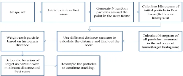
2. PARTICLE FILTER

Particle filtering has emerged recently in the domain of computer vision. The advantage of particle filter over other types of filters is that it allows for a state space representation of any kind of distribution. It also allows for linear, non-Gaussian models and processes. Particle Filter is concerned with the issue of tracking single or multiple identifiable objects. It is a conjecture tracking system that is expected to explain certain observations, that approximates the filtered

further back in positions distribution by a set of weighted particles. It weights the particles based on the likelihood score and propagates them according to the motion model used [1, 2, 3].

The two major problems addressed here to check the performance of the algorithms. The first problem addressed is the variation of different distance measures to compute the best match point. The second problem addressed is about various re-sampling methods to select and re-generate the particles which are used to keep track of the object perfectly.

3. DISTANCE MEASURES

One of the most important problem that arise throughout the world of sciences is that of deciding whether two statistical distributions are same or they differ. The process of measurement in image processing is based on the similarity of histograms. The target histogram is compared with that of other candidate histograms which are extracted from previous frame and the most similar one is chosen. The similarity measure is computed over the entire particle set. The rapport suggesting the similarity of characteristics between all pairs of particles is considered based on their distances. The similarity measure between target model and candidate model is computed by applying distance measures. The results generated by using different distance measures [4] are then compared.

In particle filter tracking, the histogram for the neighbourhood of each particle is computed. The reference histogram and target histogram are compared using suitable distance measure and arrive at the similarity score for each particle. Various Distance Measures are applied to calculate the similarity score for each particle. For each, measure a match score is computed by iteratively comparing the histograms of particles in reference image and target image.

The different distance measures used in our work are given in [4-9].

3.1 Co-relation distance

The correlation coefficient technique is adopted to reveal similarities among numerous distance/similarity measures. If the value gets close to 1, it represents a good fit. i.e. two distances measures are semantically similar. As the fit gets worse, the correlation coefficient approaches zero.

𝑑 𝐻1. 𝐻2 =

𝐻1 𝐼 − 𝐻1` 𝐻2 𝐼 . 𝐻2`

(2)

The value of „d‟ lies between 0 and 1 and for a perfect match, value of „d‟ is close to 1.

3.2 Chi-Square distance

The Euclidean distance between the components of the profiles of sample points, on which a weighting is defined (each term has a weight), is called the chi-square distance.

𝑑 𝐻1. 𝐻2 = (𝐻1 𝐼 − 𝐻2 𝐼 ) 2

𝐻1 𝐼

3.3 Bhattacharya distance

In statistics, the Bhattacharyya distance measures the similarity of two discrete or continuous probability distributions. The Bhattacharyya coefficient is an approximate measurement of the amount of overlap between two statistical samples. The coefficient can be used to determine the relative closeness of the two samples being considered.

𝑑 𝐻1. 𝐻2 = 1 −

1

𝐻1`𝐻2`𝑁2

(𝐻1 𝐼 , 𝐻2 𝐼

3.4 Intersection distance

The intersection between two probability distribution function (pdfs) is widely used form of similarity. It shows the non-overlaps between two pdfs is defined.

𝑑 𝐻1. 𝐻2 = min⁡((𝐻1 𝐼 , 𝐻2 𝐼 )

3.5 Minkowski form distance

Minkowski distance is the generalized form of city block distance coined by late Hermann Minkowski and Euclidean distance derived from Pythagorean Theorem.

d(H1,H2) = (



|

fi

(

I

)



fi

(

J

)

|

p)1/p

3.6 Swain and Ballard





 _n

n

i

J f i

J f i I f i J

I

S 1

) (

)) ( ), ( min( )

, (

3.7 Kullback-Leibler(kl) divergence

𝑑 𝑦 ≡ 𝑑 𝑝 𝑦 , 𝑞 = 𝑞𝑢𝑙𝑜𝑔

𝑞𝑢

𝑝𝑢(𝑦) 𝑚

𝑢=1

3.8 Jeffrey-divergence

Jeffrey divergence is the symmetric version of Kullback Leibler distance with respect to both q and p. The value of „d‟ lies between 0 and 1 and for a perfect match, value of „d‟ is close to 0.

3.9 Quadratic distance

 

I

J



Fi

Fj

 

Fi

Fj



D

,





T

A



The value obtained from the distance measure for every particle set is called the score. They are used to represent and predict the next match point.

4. RE-SAMPLING

Re-Sampling is used to select and re-generate the particles around the target location to keep the tracking process intact. In the set of particles under consideration, there may be few particles that move in the wrong direction. After a few iterations those particles will not contain any information about the target location. This will result in the few of particles having weights close to 0 and the rest of the particles having weights nearing 1. Because those few particles have weights close to 1, they are not enough to detect the movement of target, so algorithm may lose track of the target quickly. This is called particle degeneracy. In order to avoid this effect, the particles needs to be re-sampled at time t from the particle set, at time t+∂t with replacement of particles having low weights. The new particle set may contain multiple copies of particles with high weights whereas particles with low weights are likely to be discarded form the set. This can be done by selecting particles according to their weights [10-13].

The Re-Sampling step replaces the weighted density particle Pm to an un-weighted density particle P′m by eliminating the particles having low importance weights and by replicating those particles having high importance weights.

More formally

Pm x = wi∂(x − xi) m

i=1

Is replaced by

P′m x = 1

m∂(x − xy∗) m

≡ mi

(3)

The different Re-sampling methods are:

a. Multinomial Re-sampling

This is the simplest approach of Re-Sampling. It is based on the idea of drawing conditionally new positions independently from a certain common point distribution. Then N ordered uniform random numbers are generated and those numbers are used to select {x*y} particles according to the binomial distribution.

b. Stratified Re-sampling

In this approach of Re-Sampling, the weights are first added to get the weighted sum; it is then divided into equal pieces and is uniformly sampled on each piece. The points with large weights are sampled at least once and those particles with small weights are sampled at only once.

c. Systematic Re-sampling

In this approach of Re-Sampling, the procedure is similar to stratified re-sampling except that same uniform weights are used for each piece.

d. Residual Re-sampling

Residual Re-Sampling is also called Remainder Re-Sampling. In residual Re-Sampling the number of replicated particles is calculated first by truncation or rounding of the product w(m)M. In the case of truncation, the number of particles produced is generally less than M. So it is required to process the left over particles(residues) in order to compensate for the total number of particles.

5. COMPARASION

OF

DISTANCE

MEASURES

The distance measures mentioned in Section 3 are applied to an image set. The output of distance measure is a score. The score reveals the similarity between the selected targets. The table below gives the following details, for each distance measure the score value is computed, this is done by iteratively computing the histograms of reference image and the search image and applying the distance measure to the obtained values. The similarity between the particles can be considered with those having highest score for some of the distances and those with lowest score for other measures, mentioned in Section 3.

[image:3.595.131.440.628.756.2]

Scores are computed for all the particles generated in the subsequent frames. For each particle, corresponding score and its position is indexed. Consequently only the particles with high importance score are selected and their index is used for Re-Sampling.

Table 1. Comparing the distance measures with scores.

Sl Distance Score

1 Co-relation 0.9996

2 Chi-square 0.4535

3 Bhattacharya 0.9993

4 Intersection 0.7366

5 Minkowski form 62.960

6 Swain and ballard 0.7600 7 Jeffrey-divergence 87.9931 8 Kullback-leibler(kl) 1290.0 9 Quadratic distance 201.35

6. ALGORITHM

Input: Video/Image Sequences

Output: Particle generation, selection and tracking of the target.

Steps

i. Initialize the target in the first frame, initial position (Xt) of target.

ii. Generate a particle set of N particles {Xm t} m = 1 ….N around the object or entire frame. For t = 1,2, . . . j = 1, . . . . N, sample x_t(j)~P xt xt−1

(j)

.

iii. Calculate the histogram for all the particles and compute the match score by comparing with the reference histogram.

iv. Compute the Weights for each particle based on match score.

v. Normalize the weights {w_t j }:w_t j = wt (j)

w_t(j)

N j=1

vi. Select the location of a target as a particle with best match score

vii. A collection of samples, from which the approximate posterior distribution is computed.

viii. The mean is computed using the collection of selected samples (particles)

ix. Re-sample the particles for next iteration. Multiply/discard samples x_t(j) with high/low importance weight w_t−1(j) in order to obtain N new random samples approximately distributed according to the model.

x. Set t = t + 1 and return to step 2.

(4)

7. RESULTS AND ANALYSIS

Fig 1. Distribution of particles and nearest match points The above results show the comparison of different distances measure algorithm applied to two consecutive frames

Initial point X=132 Y=105

Bhattacharya X=114 Y=46

Chi-Square X=126 Y=113

Co-Relation X=122 Y=85

Intersection X=122 Y=85

Jeffrey-Divergence X=114 Y=46

Kull-Back X=76 Y=56

Minkowski X=122 Y=85

Quadratic X=114 Y=46

[image:4.595.321.543.61.532.2]

Swain and Ballard X=122 Y=85

Fig 2. Distribution of particles and nearest match points. The above results show the comparison of different distances measure algorithm applied to two consecutive frames.

Inital point X=176 Y=123

Bhattacharya X=176 Y=131

Chi-Square X=176 Y=149

Co-Relation X=176 Y=131

Intersection X=176 Y=131

Jeffrey-Divergence X=176 Y=149

Kull-Back X=136 Y=64

Minkowski X=176 Y=131

Quadratic X=176 Y=149

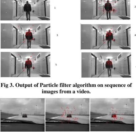
Fig 3. Output of Particle filter algorithm on sequence of images from a video.

[image:4.595.55.266.72.168.2]

Fig 3 & 4 show the use of simple random re-sampling algorithm. Fig 5 shows the use of residual re-sampling algorithm and is better compared to the results in Fig 3 and 4.

7.1 Validation of the Algorithm

[image:4.595.325.546.82.296.2] [image:4.595.59.265.222.519.2]

(5)

7.1.1 Pixel Cross-Correlation

i. Let there be a reference image A and a matched image B, for each position in A.

ii. Find the sum of square difference between pixel values.



(

A



B

)

2

iii. Find the percentage of difference in pixel value.



  B A B A Per * ) ( 2

iv. Find the accuracy by,Acc=100-Per.

7.1.2 Discrete approximate matching

ii. Find if there exists a similar point in an area of 3X3 around the corresponding point in B.

iii. Find the total number of match positions, find the accuracy.

iv. ( )_*₁₀₀

N totalmatch

Acc

7.1.3 Pixel Difference Method

ii. Find the difference in pixel values between the two images.

abs(A(i,j)-B(i,j)).

iii. Find the sum of pixel difference.

Sum=





b a

B

A

abs

,

)

(

iv. Find percentage of accuracy.

100 * 255 ) 255 ( N sum N

Acc 

Cross correlation is a standard method of estimating the degree to which two series are correlated. For all the methods considering each position in reference and matched images the above methods are used to analyze the accuracy. The analysis showed that Bhattacharya Distance, Co-Relation, Intersection gives better results for most of the image sequences. Other methods produce varying results depending on the contents of the image. It is also observed that use of the Re-Sampling methods like Residual, Stratified methods give good results for drawing and selecting particles.

Implementation details

The proposed approach is implemented on Windows 7 in Microsoft Visual Studio platform using VC++ language for programming.

8. CONCLUSION AND FUTURE

WORK

Particle filter based tracking is used to track human in indoor or outdoor environment. Particle filter algorithm is a popular substitute for the many of the filters like Kalman filter in presence of non-Guassianity of noise statistics and non-linearity of the relationships between consecutive states. The algorithm shows satisfactory results. In previous methods the algorithm uses simple distance measures and re-sampling functions for tracking but failed in certain complex situations. The parameters of the algorithm has been varied to see its functionality and its output in different cases i.e. by varying the distance measure to find out the best possible scores, nearest match points and better re-sampling methods to retain the particles. The algorithm can be further optimized to show more robustness and accuracy in tracking by integrating the model with multiple features.

9. ACKNOWLEDGEMENTS

The authors acknowledge Prof N R Shetty, Director, Nitte Meenakshi Institute of Technology and Dr H C Nagaraj, Principal, Nitte Meenakshi Institute of Technology for providing the support and infrastructure to carry out the research.

10. REFERENCES

[1] “Video Based Moving Object Tracking by Particle Filter” Md. Zahidul Islam, Chi-Min Oh and Chil-Woo Lee Chonnam National University ,International Journal of Signal Processing, Image Processing and Pattern Vol. 2, No.1, March, 2009.

[2] M. G. S. Bruno. Mixed-state particle filters for multi aspect target tracking in image sequences. In Proc. ICASSP, 2003.

[3] A Novel Particle Filter based on Propagation and PredictionBAI Xiangfeng, LI Aihua, LI Jialei, LIU Taiyang 2011 Third International Conference on Measuring Technology and Mechatronics Automation

[4] Evaluation of similarity measurement for Image retrieval Dengsheng Zhang and Guojun Lu Gippsland School of Computing and Info Tech, Monash University.

[5] The Quadratic-Chi Histogram Distance Family. Ofir Pele and Michael Werman School of Computer Science, The Hebrew University of Jerusalem.

[6] The computation of the bhattacharyya distance between histograms without histograms S´everine Dubuisson Laboratoire d‟Informatique de Paris 6, Universit´e Pierre et Marie Curie.

[7] The Bhattacharyya Metric as an Absolute Similarity Measure for Frequency Coded Data.N. A. Thacker, F. J. Aherne and P. I. Rockett Tina Memo No. 1997-001 Presented at: TIPR‟97, Prague 9-11 June, 1997.and publiseed in Kybernetika, 34, 4, 363-368, 1997.

(6)

Second International Conference on Innovations in Information Technology (IIT‟05).

[9] Color Matching of Images by using Minkowski- Form DistanceBy Ajay B. Kurhe, Suhas S. Satonka, Prakash B. Khanale Global Journal of computer science and technology, Volume 11 Issue 5 Version 1.0 April 2011.

[10]“Comparison of Resampling Schemes for Particle Filtering Randal Douc, Olivier Cappé, Eric Moulines, GET Télécom Paris 46 rue Barrault, 75634 Paris, 2010, France.

[11]ON RESAMPLING ALGORITHMS FOR PARTICLE FILTERS “Jeroen D. Hol, Thomas B. Sch¨on, Fredrik

Gustafsson, Division of Automatic Control Department of Electrical Engineering Link¨oping University SE-581 83, Link¨oping, 2008 Sweden.

[12]Resampling Algorithms for Particle Filters: A Computational Complexity PerspectiveMiodrag Boli´c Petar M. Djuri´c Sangjin Hong Department of Electrical and Computer Engineering, Stony Brook University Stony Brook, New York 11794, USA