A fast and accurate FFT based method for pricing early exercise options under Lévy processes

A fast and accurate FFT-based method

for pricing early-exercise options under

Lévy processes

Lord, Roger and Fang, Fang and Bervoets, Frank and

Oosterlee, Kees

Rabobank International, Delft University of Technology and Center

for Mathematics and Computer Science (CWI), Amsterdam

28 February 2007

Online at

https://mpra.ub.uni-muenchen.de/1952/

EARLY-EXERCISE OPTIONS UNDER L´EVY PROCESSES

R. LORD∗_{, F. FANG}†_{, F. BERVOETS}‡_{, AND C.W. OOSTERLEE}§

Abstract. A fast and accurate method for pricing early exercise and certain exotic options in computational finance is presented. The method is based on a quadrature technique and relies heavily on Fourier transformations. The main idea is to reformulate the well-known risk-neutral valuation formula by recognising that it is a convolution. The resulting convolution is dealt with numerically by using the Fast Fourier Transform (FFT). This novel pricing method, which we dub the Convolution method, CONV for short, is applicable to a wide variety of payoffs and only requires the knowledge of the characteristic function of the model. As such the method is applicable within exponentially L´evy models, including the exponentially affine jump-diffusion models. For an M-times exercisable Bermudan option, the overall complexity isO(M Nlog(N)) withN grid points used to discretise the price of the underlying asset. It is shown how to price American options efficiently by applying Richardson extrapolation to the prices of Bermudan options.

Key words. option pricing , Bermudan options, American options, convolution, L´evy Pro-cesses, Fast Fourier Transform

AMS subject classifications. 65Y20, 65T50, 62P05, 60E10, 91B28

Preferred short title : CONV method for option pricing

1. Introduction. When valuing and risk-managing exotic derivatives, practi-tioners demand fast and accurate prices and sensitivities. As the financial models and option contracts used in practice are becoming increasingly complex, efficient methods have to be developed to cope with such models. Aside from non-standard exotic derivatives, plain vanilla options in many stock markets are actually of the American type. As any pricing and risk management system has to be able to calibrate to these plain vanilla options, it is of the utmost importance to be able to value these American options quickly and accurately.

By means of the risk-neutral valuation formula the price of any option without early exercise features can be written as an expectation of the discounted payoff of this option. Starting from this representation one can apply several numerical techniques to calculate the price itself. Broadly speaking one can distinguish three types of methods: Monte Carlo simulation, numerical solution of the corresponding partial-(integro) differential equation (P(I)DE) and numerical integration. While the treatment of early exercise features within the first two techniques is relatively standard, the pricing of such contracts via quadrature pricing techniques has not been considered until recently, see [1, 32]. Each of these methods has its merits and demerits, though for the pricing of American options the PIDE approach currently seems to be the clear favorite [19, 34].

In the past couple of years a vast body of literature has considered the mod-eling of asset returns as infinite activity L´evy processes, due to the ability of such processes to adequately describe the empirical features of asset returns and at the same time provide a reasonable fit to the implied volatility surfaces observed in op-tion markets. Valuing American opop-tions in such models is however far from trivial,

∗_{Financial Engineering (UC-R-380), Rabobank International, P.O. Box 17100, Utrecht, The}

Netherlands, e-mail: [email protected]

†_{Delft University of Technology, Delft Institute of Applied Mathematics, Delft, the Netherlands,}

email: [email protected],

‡_{Modelling and Research (TC 2121), Rabobank International, Thames Court, 1 Queenhithe,}

London EC4V 3RL, UK, e-mail: [email protected],

§_{CWI – Center for Mathematics and Computer Science, Amsterdam, the Netherlands, email:}

[email protected], and Delft Institute of Applied Mathematics, Delft University of Technology.

due to the weakly singular kernels of the integral terms appearing in the PIDE, as reported in, e.g., [3, 4, 11, 20, 28, 33].

In this paper we present a novel quadrature-based method for pricing options with early exercise features. The method effectively combines the recent quadrature pricing methods of [1] and [32] with the methods based on Fourier transformation pioneered by [8, 29, 26]. Though the transform methods so far have mainly been used for the pricing of European options, we show how early exercise features can be incorporated naturally. The only requirement of the method is that the condi-tional characteristic function of the underlying asset is known, which is the case for many exponential L´evy models, with the popular exponentially affine jump-diffusion (EAJD) models of [13] as an important subclass. In contrast to the PIDE methods, processes of infinite activity, such as the Variance Gamma (VG) or CGMY models can be handled with relative ease. In addition to its flexibility, a real benefit of our method is its impressive computational speed, as all integrations can be evaluated using the FFT algorithm.

This paper is organized as follows. We start with an overview of the recent history of the FFT in option pricing. Subsequently we introduce the novel method called Convolution (CONV) method for early exercise options. Its high accuracy and speed are demonstrated by pricing several Bermudan and American options under Geometric Brownian Motion (GBM), VG and CGMY.

2. Overview Transform and Quadrature Pricing Methods. All trans-form methods depart from the risk-neutral valuation trans-formula that, for a European option, reads:

V(t, S(t)) =e−rτ_{E[V(T, S(T))], (1)}

whereV denotes the value of the option,ris the risk-neutral interest rate,tis the current time point, T is the maturity of the option and τ =T −t. The variable

S denotes the asset on which the option contract is based. The expectation is taken with respect to the risk-neutral probability measure. Although we assume throughout the paper that interest rates are deterministic, this assumption can be relaxed at the cost of increasing the dimensionality of some of the methods. As (1) is an expectation, it can be calculated via numerical integration provided that the probability density is known in closed-form.

This is not the case for many models which do however have a characteristic function in closed form.1 _{A number of papers starting from Heston [18] have}

at-tacked the problem via another route. Focusing on a plain vanilla European call option, note that (1) can be written very generally as:

V(t, S(t)) =e−rτ_{(F(t, T)·∆−K·P(S(T)> K)), (2)}

whereF(t, T) is the forward price of the underlying asset at timeT, as seen fromt,

P(S(T)> K) is the risk-neutral probability of ending up in-the-money and ∆ is the delta of the option, the sensitivity of the option with respect to changes in the un-derlying. Note that (2) has the same form as the celebrated Black-Scholes formula. The delta can be interpreted as the probability of ending up in the money under the stock price measure, induced by taking the asset price itself as the numeraire asset. As such, both these cumulative probabilities can be found by inverting the characteristic function, an approach which in the form used here dates back to

1

Gurland [17] and Gil-Pelaez [16]. We can write:

P(ST > K)= 1

2+ 1 2π

Z ∞

−∞

e−iuk_φ(u)

iu du, (3)

∆ = 1

2+ 1 2π

Z ∞

−∞

e−iuk_φ(u−i)

iuφ(−i) du, (4)

whereiis the imaginary unit,kis the logarithm of the strike priceKandφis the characteristic function of the log-underlying, i.e.,

φ(u) =EheiulnS(T)i_.

Carr and Madan [8] considered another approach. Note that L1_{-integrability is a}

sufficient condition for the Fourier transform of a function to exist. A call option is certainly notL1_{-integrable with respect to the logarithm of the strike price, as:}

lim

k→−∞V(t, S(t)) =S(t),

Damping the option price with exp (αk) for α > 0 solves this however, and Carr and Madan ended up with:

F {eαkV(t, k)}=e−rτ

Z ∞

−∞

eiukE(S(T)−ek)+dk

= e

−rτ_{φ(u−(α+ 1)i)}

−(u−αi)(u−(α+ 1)i), (5)

where with abuse of notation we now consider the option priceV as a function of time and k. Though this approach was new to mathematical finance, the idea of damping functions on the positive real line in order to be able to find their Fourier transform dates back to at least Dubner and Abate [12].

A necessary and sufficient condition for (5) to exist is that

φ(−(α+ 1)i) =E[S(T)α+1]<∞,

i.e., that the (α+ 1)th moment of the asset price exists. The option price can subsequently be recovered by inverting (5) and undamping

V(t, k) = 1 2πe

−rτ−αk

Z ∞

−∞

e−iuk φ(u−(α+ 1)i)

−(u−αi)(u−(α+ 1)i)du (6)

The representation in (6) has two distinct advantages over (3). Firstly, it only re-quires one numerical integration. Secondly, whereas (2) can suffer from cancellation errors, the numerical stability of (6) can be controlled by means of the damping co-efficientα. Finally we note that if we discretise (6) with Newton-Cˆotes quadrature the option price can very efficiently be evaluated by means of the FFT, yielding option prices over a whole range of strike prices.

The methods considered up till here can only handle the pricing of European options. Before turning to methods that can handle early exercise features, let us introduce some notation. We define the set of exercise dates asT ={t1, . . . , tM}and

0 =t0≤t1. For ease of exposure we assume the exercise dates are equally spaced,

so that tm+1−tm = ∆t. The best known examples of options with early exercise

holder of the option obtains the exercise payoffE(t, S(t)). The Bermudan option price can then be found via backward induction as

  

V(tM, S(tM)) = E(tM, S(tM))

C(tm, S(tm)) = e−r∆tEtm[V(tm+1, S(tm+1))]

V(tm, S(tm)) = max{C(tm, S(tm)), E(tm, S(tm))},

m=M −1, . . . ,1, (7)

with C the continuation value of the option and V the value of the option im-mediately before the exercise opportunity. Note that we now explicitly attached a subscript to the expectation operator to indicate that the expectation is being taken with respect to all information available at timetm.

Clearly the dynamic programming problem in (7) is a successive application of the risk-neutral valuation formula, as we can write the continuation value as

C(tm, S(tm)) =e−r∆t

Z ∞

−∞

V(tm+1, y)f(y|S(tm))dy, (8)

wheref(y|S(tm)) represents the probability density describing the transition from

S(tm) attmtoy attm+1. Based on (7) and (8) the QUAD method was introduced

in [1]. The method requires the transition density to be known in closed-form, which is the case in e.g. the Black-Scholes model and Merton’s jump-diffusion model. This requirement is relaxed in [32], where the QUAD-FFT method is introduced. The underlying idea is that the transition density can be recovered by inverting the characteristic function, opening up the QUAD method to a much wider range of models. As such the QUAD-FFT method effectively combines the QUAD method with the early transform methods. The overall complexity of both methods is

O(M N2_{) for anM-times exercisable Bermudan option withN grid points used to}

discretise the price of the underlying asset.

The complexity of this method can be improved toO(M Nlog(N)) if the under-lying is a monotone function of a L´evy process. We will demonstrate this shortly. In the remainder we assume, as is common, that the underlying process is modelled as an exponential of a L´evy process. Letx1, . . . , xN be a uniform grid for the log-asset

price. If we discretise (8) by the trapezoidal rule we can write the continuation value in matrix form as

C(tm)≈e−r∆t∆x

FV−1

2(V (tm+1, x1)f1+V(tm+1, xN)fN)

, (9)

where

fi =

  

f(xi|x1)

.. .

f(xi|xN)

 

, F= (f₁, . . . ,f_N), V=   

V(tm+1, x1)

.. .

V(tm+1, xN)

  ,

andf(y|x) now denotes the transition density in logarithmic coordinates. The key observation is that the increments of L´evy processes are independent, so that due to the uniform grid

Fj,ℓ=f(yj|yℓ) =f(yj+1|yℓ+1) =Fj+1,ℓ+1; (10)

The previous strain of literature does not seem to have picked up on a presen-tation by Reiner [30], where it was recognised that for the Black-Scholes model the risk-neutral valuation formula in (8) can be seen as a convolution or correlation of the continuation value with the transition density. As convolutions can be handled very efficiently by means of the FFT, an overall complexity of O(M NlogN) can be achieved. By working forward instead of backward in time a number of discrete path-dependent options can also be treated, such as lookbacks, barriers, Asian op-tions and cliquets. Building on Reiner’s idea, Broadie and Yamamoto [6] have been able to reduce the complexity toO(M N) for the Black-Scholes model by combining the double-exponential integration formula and the Fast Gauss Transform. Nat-urally their technique is applicable to any model in which the transition density can be written as a weighted sum of Gaussian densities, which is the case in e.g. Merton’s jump-diffusion model.

As one of the defining properties of a L´evy process is that its increments are independent of each other, the insight of Reiner has a much wider applicability than only to the Black-Scholes model. This is especially appealing since the usage of L´evy processes in finance has become more established nowadays. By combining Reiner’s ideas with the work of Carr and Madan, we introduce the Convolution method, or CONV method for short. The complexity of the method is O(M NlogN) for an

M-times exercisable Bermudan option.

3. The CONV Method. The main premise of the CONV method is that the conditional probability densityf(y|x) in (8) only depends onxandy via their difference

f(y|x) =f(y−x). (11)

Note that x and y do not have to represent the asset price directly, they could be monotone functions of the asset price. The assumption made in (11) therefore certainly holds when the asset price is modelled as a monotone function of a L´evy process, since one of the defining properties of a L´evy process is that its increments are independent of each other. As mentioned earlier, we choose to work with ex-ponential L´evy models in the remainder of this paper. In this casexand yin (11) represent the log-spot price. Let us see what the impact of independent increments is on the continuation value in (8). By including (11) in (8) and changing variables

z=y−xthe continuation value can be expressed as

C(tm, x) =e−r∆t

Z ∞

−∞

V(tm+1, x+z)f(z)dz, (12)

which is a cross-correlation2 _{of the option value at time t}

m+1 and the density

f(z), or equivalently, a convolution ofV(tm+1) and the conjugate of f(z). If the

density function has an easy closed-form expression, it may be beneficial to proceed along the lines of (9). However, for many exponential L´evy models we either do not have a closed-form expression for the density (e.g. the CGMY/KoBoL model of [5] and [7] and many EAJD models), or if we have, it involves one or more special functions (e.g. the VG model). In contrast, the characteristic function of the log-spot price can typically be found in closed-form or, in case of the EAJD models, via the solution of a system of ODEs.

2

The cross-correlation of two functionsf(t) andg(t), denotedf ⋆ g, is defined by

f ⋆ g≡f¯(−t)∗g(t) =

Z ∞ −∞

f(τ)g(t+τ)dτ,

Let us therefore take the Fourier transform of (12). The insight that the contin-uation value can be seen as a convolution is particularly useful here, as the Fourier transform of a convolution is merely the product of the Fourier transforms of the two functions being convolved. In the remainder we will employ the following definitions for the continuous Fourier transform and its inverse,

ˆ

h(u) :=F {h(t)}(u) = Z ∞

−∞

eiuth(t)dt, (13)

h(t) :=F−1{hˆ(u)}(t) = 1 2π

Z ∞

−∞

e−iuthˆ(u)du. (14)

If we dampen the continuation value (12) by a factor exp (αx) and subsequently take its Fourier transform, we arrive at

er∆t_{F {c(t}

m, x)}(u) =

Z ∞

−∞

eiux_eαx

Z ∞

−∞

V(tm+1, x+z)f(z)dzdx (15)

= Z ∞

−∞

Z ∞

−∞

eiu(x+z)v(tm+1, x+z)e−iz(u−iα)f(z)dzdx.

where in the first step we used the risk-neutral valuation formula from (12). We introduced the convention that small letters indicate damped quantities, i.e.,

c(tm, x) =eαxC(tm, x) andv(tm, x+z) =eα(x+z)V(tm, x+z). Changing the order

of integration and remembering thatx=y−z, we obtain

er∆t_{F {c(t}

m, x)}(u) =

Z ∞

−∞

Z ∞

−∞

eiuy_v(t

m+1, y)dy e−i(u−iα)zf(z)dz

= Z ∞

−∞

eiuyv(tm+1, y)dy

Z ∞

−∞

e−i(u−iα)zf(z)dz

=F {eαyV(tm+1, y)}(u)φ(−(u−iα)). (16)

In the last step we used the fact that the complex-valued Fourier transform of the density is simply the extended characteristic function

φ(x+yi) = Z ∞

−∞

ei(x+yi)z_{f(z)dz, (17)}

which is well-defined whenφ(yi)<∞, as|φ(x+yi)| ≤ |φ(yi)|. As such (16) puts a condition on the damping coefficientα, becauseφ(αi) must be finite.

The difference with the Carr-Madan approach in (5) is that we take a transform with respect to the log-spot price instead of the log-strike price, something which [26] and [29] also consider for European option prices. The damping factor is again certainly necessary when considering e.g. a Bermudan put, as thenV(tm+1, x) tends

to a constant when x→ −∞, and as such is notL1-integrable. For the Bermudan put we must choose α >0. Though other values ofαare allowed in principle, we need to know the poles of the payoff-transform in order to apply Cauchy’s residue theorem, see e.g. [23] and [24]. This restriction onαwill disappear when we switch to a discretised version of (16) in the next section. The Fourier transform of the damped continuation value can thus be calculated as the product of two functions, one of which, the extended characteristic function, is readily available in exponential L´evy models. How we proceed should be fairly clear. We recover the continuation value by taking the inverse Fourier transform of the right-hand side of (16), and calculateV(tm) as the maximum of the continuation and the exercise value attm.

We repeat (7) recursively until we have obtained the option price at time t0. In

Algorithm 1: The CONV algorithm for Bermudan options

V(tM, x) =E(tM, x) for allx

Form=M−1 to 0

DampenV(tm+1, x) with exp(αx) and take its Fourier transform

Calculate the right-hand side of (16)

CalculateC(tm, x) by applying Fourier inversion to (16) and undamping

V(tm, x) = max{(E(tm, x), C(tm, x)}

Nextm

In Appendix A we demonstrate how the hedge parameters can be calculated in the CONV method. As differentiation is exact in Fourier space, they will be more stable than when calculated via finite-difference based approximations.

The following section deals with the implementation of the CONV algorithm. In particular we employ the power of the FFT to approximate the continuous Fourier transforms that are involved.

4. Implementation Details of the CONV Method. The very essence of the CONV method is the calculation of a convolution3_:

c(x) = 1 2π

Z ∞

−∞

e−iuxˆv(u)φ(−(u−iα))du, (18)

where ˆv(u) is the Fourier transform ofv:

ˆ

v(u) = Z ∞

−∞

eiuyv(y)dy. (19)

In the remainder of this section we will just focus on equations (18) and (19) for notational ease. In order to be able to use the FFT for exponentially affine models means that we have to switch to logarithmic coordinates. For this reason the state variables x and y will represent lnS(tm) and lnS(tm+1), up to a constant shift.

This section is organised as follows. Section 4.1 deals with the discretisation of the convolution in (18) and (19). Section 4.2 analyses the error made by one step of the CONV method and provides guidelines to choosing the grids for u, x and y. Section 4.3 considers the choice of grid further and investigates how to deal with points of discontinuity. This will prove to be very important if we want to guarantee a smooth convergence of the algorithm. Finally, sections 4.4 and 4.5 deal with the pricing of Bermudan and American options with the CONV method.

4.1. Discretising the Convolution. We approximate both integrals in (18) and (19) by a discrete sum, so that the FFT algorithm can be employed for their computation. This necessitates the use of uniform grids foru, xandy:

uj =u0+j∆u, xj =x0+j∆x, yj =y0+j∆y, (20)

wherej= 0, . . . , N−1. Though they may be centered around a different point, the

x- andy-grids have the same mesh size: ∆x= ∆y. Further, the Nyquist relation must be satisfied, i.e.,

∆u·∆y= 2π

N. (21)

In principle we could use the Fractional FFT algorithm (FrFT) which does not require the Nyquist relation to be satisfied. Numerical tests indicated that the FrFT is on average 4 times slower than the FFT, and that we could obtain a

3

similar accuracy by quadrupling the number of points, so that we opted to use the FFT throughout. Details about the exact location of x0 and y0 will be given in

Section 4.3, as will details about the range of all grids. Inserting (19) into (18), and approximating (19) with a general Newton-Cˆotes rule and (18) with the left-rectangle rule yields:

c(xp)≈

∆u∆y

2π

N_X−1

j=0

e−iujxp_φ(−(u

j−iα)) N_X−1

n=0

wneiujynv(yn), (22)

forp= 0, . . . , N−1. When using the trapezoidal rule we choose the weightswn as:

w0= 1

2, wN−1= 1

2, wn= 1 forn= 1, . . . , N−2. (23) Though it may seem that the choice for the left-rectangle rule in (18) would cause the leading error term in (22) to be O(du), the error analysis will show that the Newton-Cˆotes rule one uses to approximate (19) is one of the main determinants hereof. Inserting the definitions of our grids into (22) yields:

c(xp)≈

e−iu0(x0+p∆y)

2π ∆u

N_X−1

j=0

e−ijp2π/Neij(y0−x0)∆u_φ(−(u

j−iα)) ˆv(uj), (24)

where the Fourier transform ofv is approximated by:

ˆ

v(uj)≈eiu0y0∆y N_X−1

n=0

eijn2π/Neinu0∆y_w

nv(yn). (25)

Let us now define the DFT and its inverse of a sequencexp, p= 0, . . . , N−1,as:

Dj{xn}:= N_X−1

n=0

eijn2π/Nxn, Dn−1{xj}=

1

N

N_X−1

j=0

e−ijn2π/Nxj. (26)

Though the reason why will become clear later, let us set u0 = −N/2∆u. As

einu0∆y _{= (−1)}n _{this finally leads us to write (24), (25) as:}

c(xp)≈eiu0(y0−x0)(−1)pD−1p {eij(y0−x0)∆uφ(−(uj−iα))Dj{(−1)nwnv(yn)}}.

(27)

4.2. Error Analysis of the CONV Method. A first inspection of (27) sug-gests that error will arise from two sources:

- Discretisation of both integrals in (18) and (19); - Truncation of these integrals.

approach infinity. We depart from the risk-neutral valuation formula with damping and without discounting:

c(x) = Z ∞

−∞

v(x+z)e−αzf(z)dz. (28)

The first approximation we make is due to replacingvby its Fourier series expansion on [−L/2, L/2], where we have fixedL >0:

e

c1(x)≈

Z ∞

−∞ ∞

X

j=−∞

vjeij2π(x+z)/Le−αzf(z)dz=

∞

X

j=−∞

vjeij2πx/Lφ

−(j2π

L −iα)

,

(29) using the dominated convergence theorem. The Fourier series coefficients of v are given by:

vj=

1

L

Z L/2 −L/2

v(y)eij2πy/Ldy. (30)

As the Fourier series expansion of v is a periodic function with period L, only agreeing withv on [−L/2, L/2], the error from this approximation equals:

e1(L) =ec1(x)−c(x)

= Z

IR\[−L/2,L/2]



v(x+z)− ∞

X

j=−∞

vjeij2π(x+z)/L



e−αzf(z)dz. (31)

A general guideline for choosing L is to ensure that the mass of the density out-side [−L/2, L/2] is negligible. The function ec1 can, at least on this interval, be

interpreted as an approximate Fourier series expansion ofc(x).

The second error arises by truncating the infinite summation from −N/2 to

N/2−1, leading toec2 and its associated errore2:

e

c2=

N/2−1

X

j=−N/2

vje−ij2πx/Lφ

−(j2π

L −iα)

,

|e2(L, N)|=|ec1(x)−ec2(x)| ≤ ∞

X

|j|=N/2 |vj||φ

−(j2π

L −iα)

|. (32)

To further bound this error we require knowledge about the rate of decay of Fourier coefficients. It is well known that even if v is only piecewise C1 _{on [−L/2, L/2]}

its Fourier series coefficients vj tend to zero as j → ±∞. The modulus ofvj can

therefore be bounded as:

|vj| ≤ η1(L)

|j|β1 . (33)

Byηi(·) we denote a bounding constant. The quantities it depends on are between

brackets. For functions that are piecewise continuous on [−L/2, L/2] but whose

L-periodic extension is discontinuous, we typically have β1 = 1 as the following

example demonstrates.

Example 4.2.1 (European Put). Suppose that we have a European put payoff and that y= lnS(t)−lnK. Then the payoff function equalsv(y) =eαy_K(1−ey₎+

and its Fourier series coefficients equal:

vj =K

e−Lα/2(−1)j e

−L/2₋₁

L(α+ 1) + 2πij −L

e−Lα/2₍₋₁₎j₋₁

(L(α+ 1) + 2πij)(Lα+ 2πij)

Clearly, β1 = 1 in (33), though when L → ∞ and j2π/L → u it can be shown

that the Fourier series coefficient converges to the Fourier transform of the payoff function, which can be seen to beO(u−2_{)from (5).}

The characteristic function can always be assumed to have power decay:

|φ(x+yi)| ≤η2(y)

|x|β2. (35)

This is overly conservative for e.g. the Black-Scholes model, where the characteristic function of the log-underlyingφ(x+yi) decays as exp(−cx2), or the Heston model where the characteristic function has exponential decay. For the most popular L´evy models however the power decay assumption is appropriate. The VG model for example hasβ2= 2τ /ν withτ being the time step. Using (33) and (35) yields:

|e2(L, N)| ≤ ∞

X

|j|=N/2

η1(L) |j|β1

η2(α) 2π

L

β2 |j|β2

≤η3(α, L)

Z ∞

N/2−1

x−β1−β2

dx

=η3(α, L)

(N/2−1)1−β1−β2

β1+β2−1

, (36)

whereη3(α, L) = 2η1(L)η2(α)(2π/L)−β2. We finally arrive at the discretised CONV

formula in (27) by approximating the Fourier series coefficients ofv in (32) with a Newton-Cˆotes rule:

e

v(uj) = 1

L∆y

N_X−1

n=0

wneiujynv(yn). (37)

This is equal to the right-hand side of (24) multiplied by 1/L. It becomes clear that we can set ∆y=L/N andy0=−L/2.

Inserting (37) in_ec2 results in the third and final approximation:

e

c3(x) =

N/2−1

X

j=−N/2

e

v(uj)e−ij2π/Lxφ

−(j2π

L −iα)

. (38)

Assuming that the chosen Newton-Cˆotes rule is ofO(N−β3_{), one can bound:}

|vj−ev(uj)| ≤

η4(α, L)

Nβ3 , (39)

leading to the following error estimate forβ26= 1:

|e3(L, N)|=|ec2(x)−ec3(x)| ≤ η4(α, L)

Nβ3

N/2−1

X

j=−N/2 |φ

−(j2π

L −iα)

|

≤η4(α, L)

Nβ3 

3φ(iα) + 2η2(α)

2π

L

−β2N/X2

j=2

1 |j|β2

 

=η5(α, L)

Nβ3 +

η6(α, L)

(1−β2)Nβ3

2β2−1

Nβ2−1−1

. (40)

with η5(α, L) = 3η4(α, L)φ(iα) and η6(α, L) = 2η2(α)η4(α, L)(2π/L)−β2. For

β2 = 1 the second error term should of course beη6(α, L) lnN/2/Nβ3.

be bounded as:

|c(x)−ec3(x)| ≤ |c(x)−ec1(x)|+|ce1(x)−ec2(x)|+|ec2(x)−ec3(x)| ≤e1(L) +e2(L, N) +e3(L, N)

=e1(L) +O(N−min (β3,β2+β3−1,β1+β2−1)) (41)

As demonstrated, in most applications β1 = 1. This implies that, aside from the

truncation error, the order of convergence will be:

- O(N−β3_{) for characteristic functions decaying faster than a polynomial;} - O(Nmin (β3,β2+β3−1,β1+β2−1)_{) for characteristic functions with power decay.} The magnitude ofβ3will depend on the interplay between the chosen Newton-Cˆotes

rule and the nature of the payoff function. One final word should be mentioned on the damping coefficientα. In the continuous version of the algorithm in Section 3α

was chosen such that the damped continuation value wasL1_{-integrable. The direct}

construction of the discretised CONV formula in Section 4.2 via a Fourier series expansion of the continuation value replacesL1_{-integrability on (−∞,∞) withL}1

-summability on [−L/2, L/2], so that the restriction on αis removed. In principle any value ofαis allowed as long asφ(iα) is finite. Nevertheless it seems sensible to adhere to the guidelines stated before, as the function will resemble its continuous counterpart more and more asLincreases. The impact ofαon the accuracy of the CONV algorithm is investigated in Section 5.1.

This concludes the error analysis of one step of the CONV algorithm. It is easy to show that the error is not magnified further in the remaining time steps. The leading error of our algorithm is therefore dictated by the time step where the order of convergence in (41) is the smallest.

4.3. Dealing with Discontinuities. Our focus in this section lies on achiev-ing smooth convergence for the CONV algorithm. As numerical experiments have shown that it is difficult to achieve smooth convergence with high order Newton-Cˆotes rules, we will from here on focus on the second order trapezoidal rule in (23). Smooth convergence is desirable as we will be using extrapolation techniques later on to price American options in Section 4.5.

The previous section analysed the error in the discretised CONV formula when we use a Newton-Cˆotes rule to integrate the functionV, the maximum of the con-tinuation value and the exercise value. If we focus on a simple Bermudan put it is clear that already at the last time step this function will have a discontinuous first derivative. Certainly it is also possible thatV itself is discontinuous, think of contracts with a barrier clause. This will affect the order of convergence.

It is well-known that if we want to numerically integrate a function with (a finite number of) discontinuities, we should split up the integration domain such that we are only integrating continuous functions. Appendix B demonstrates this for the trapezoidal rule. In particular, we show that the trapezoidal rule remains second-order if only the first derivative of the integrand is discontinuous, at the cost of non-smooth convergence. If the integrand itself is discontinuous, the trapezoidal rule loses an order. Smooth second-order convergence can be restored by placing the discontinuities on the grid. This notion has often been utilised in lattice-based techniques, though the solutions have more often than not been payoff-specific. An approach that is more or less payoff-independent was recently proposed in [22], generalising previous work by [23], which essentially places discontinuities on the grid. Unfortunately, we cannot use their methodology here, as our desire to use the FFT binds us to a uniform grid.

basic CONV algorithm. Equating the grids forxandyfor now we have:

uj= (j−n

2)∆u, xj=yj = (j− 1

2)∆y, j= 0, . . . , N−1.

Here x and y represent, up to a constant shift, lnS(tm) and lnS(tm+1),

respec-tively. If in particularx= lnS(tm)−lnS(0) andy= lnS(tm+1)−lnS(0), so that

xand y represent total log-returns, we will refer to this discretisation as Discreti-sation I. A convenient property of this discretiDiscreti-sation is that the spot price always lies on the grid, so that no costly interpolation is required to back out the desired option value. Note that we need to ensure that the mass of the density ofxandy

outside [−L/2, L/2] is negligible. Though more sophisticated approximations can be devised, we use a rule of thumb from [32] which choosesLas a multiple of the standard deviation of lnS(tm), i.e.,

L=δ· s

− ∂ 2_φ(t

m, u)

∂u2

u=0

+

∂φ(tm, u)

∂u

u=0

2

(42)

where φ(tm, u) is the characteristic function of lnS(tm) conditional upon lnS(0),

and δ is a proportionality constant. Note that there is a trade-off in the choice of L: as we set ∆y = L/N, the Nyquist relation implies ∆u = 2π/L and hence [u0, uN−1] = [−N π/L,(N−2)π/L]. Though larger values ofLimply smaller

trun-cation errors, they also cause the range of the grid in the Fourier domain to be smaller, so that the error in turn will be larger initially.

It is easy to come up with a choice of grid that allows us to place one disconti-nuity on the grid. Suppose that at timetmthe discontinuity we would like to place

on the grid isdm. We can then shift our grid by a small amount to arrive at:

xj =ǫx+ (j−L

2)∆y, yj=ǫy+ (j−

L

2)∆y, (43)

whereǫx=dm− ⌈dm/∆x⌋·∆xandǫy is chosen in a similar fashion. This

discretisa-tion will be referred to as Discretisadiscretisa-tion II. Even for plain vanilla European opdiscretisa-tions where only one time step is required this is very useful. By choosingǫy= lnK/S(0)

andǫx= 0 we ensure that the discontinuity of the call or put payoff lies on the y

-grid, and the spot price lies on thex-grid. When more discontinuities are present it seems impossible to guarantee smooth convergence without abandoning the restric-tion of a uniform grid. In order to still be able to use the computarestric-tional speed of the FFT we will then have to resort to e.g. the discontinuous FFT algorithm of [14] or a recent transform inversion technique in [24]. These directions are left for further research. Luckily, Discretisation II is well-suited for the pricing of Bermudan and American options, as we will show in the following sections.

4.4. Pricing Bermudan Options. As mentioned, when pricing Bermudan options the functionV in (7) will have a discontinuous first derivative. Though at the final exercise timetM the location of this discontinuity is known, this is not the

case at previous exercise times. All we know after calculatingV by equation (7) is that the discontinuity is contained in an interval of width ∆x, say [xℓ, xℓ+1].

If we proceed with the CONV algorithm without placing the discontinuity on the grid, the algorithm will display a non-smooth convergence. Andricopoulos et al. [1] overcome this problem by equating the exercise payoff and the continuation value, and solving numerically for the location of the discontinuity. In our framework this can be quite costly, so that we propose an effective alternative. We can use a simple linear interpolation to locate the discontinuity, saydm:

dm≈ xℓ+1(C(tm, xℓ)−E(tm, xℓ))−xℓ(C(tm, xℓ+1)−E(tm, xℓ+1))

(C(tm, xℓ)−E(tm, xℓ))−(C(tm, xℓ+1)−E(tm, xℓ+1))

In the actual implementation we will use a cubic, instead of a linear interpolation. As in Discretisation II we can now shift the grid such that dm lies on it, and

recalculate both the continuation and the exercise value. In particular, note that the inner DFT of (27) does not have to be recalculated, the only term that is affected is the outer inverse DFT. As a by-product, calculating dm automatically gives us

an approximation of the exercise boundary.

It is demonstrated in Appendix B that if we opt for the trapezoidal rule a linear interpolation is sufficient to guarantee a smooth convergence. Obviously, if higher-order Newton-Cˆotes rules are used, higher order interpolation schemes will have to be employed to locate the discontinuity. The resulting algorithm we use to value Bermudan call or put options with a fixed strikeK is presented below in pseudo-code.

Algorithm 2: Details of the algorithm for valuing Bermudan options. Ensure that the strikeK lies on the grid by settingǫy= lnK/S(0)

Form=M−1 to 1

Equate thex-grid attmto they-grid attm+1

ComputeC(tm, x) through (27)

Locatexℓ andxℓ+1 and approximatedm, e.g. via (44)

Setǫx=dmand recomputeC(tm, x)

CalculateV(tm, x) = max (E(tm, x), C(tm, x))

Set they-grid attm to be equal to thex-grid attm

Nextm

Setǫx= 0 such that the initial spot price lies on the grid

ComputeV(0, x) =C(0, x) using (27)

4.5. Pricing American Options. Within the CONV algorithm there are two ways to value an American option. One way is to approximate an American option by a Bermudan option with many exercise opportunities, the other is to use Richardson extrapolation on a series of Bermudan options with an increasing number of exercise opportunities. The method we use has been described in detail by Chang, Chung, and Stapleton [10], though the approach in finance dates back to Geske and Johnson [15]. The QUAD method in [1] also uses the same technique to price American options. We restrict ourselves to the essentials here. Let V(∆t) be the price of a Bermudan option with a maturity ofT years where the exercise dates are ∆tyears apart. It is assumed thatV(∆t) can be expanded as

V(∆t) =V(0) +

∞

X

i=1

ai(∆t)γi, (45)

with 0< γi < γi+1. V(0) is the price of the American option. Classical

extrapola-tion procedures assume that the exponentsγiare known, which means that we can

use n+ 1 Bermudan prices with varying ∆t in order to eliminatenof the leading order terms in (45). The only paper considering an expansion of the Bermudan option price in terms of ∆t we are aware of is of Howison [21], who shows that

γ1= 1 for the Black-Scholes model. Nevertheless, numerical tests indicate that the

assumptionγi=iproduces satisfactory results for the L´evy models we consider.

is either obtained via another numerical scheme, or via the CONV algorithm with 220 _{grid points. In the tables to follow we will also present the error convergence}

defined as the absolute value of the ratio between two consecutive errors. A factor of 4 then denotes second order convergence. All single-asset tests were performed in Matlab 7.0.1 on an Intel Xeon CPU 5160, 3.00GHz with 2GB RAM. The multi-asset calculations were done inCon a 64-bit machine, with a 1 GHz Bus frequency and 8GB RAM.

5.1. Characteristic Function for L´evy Price Processes. The CONV method, as outlined in Section 3, is particularly well-suited for exponential L´evy models whose characteristic functions are available in closed-form. We will briefly review some defining properties of these models before turning to the extended CGMY/KoBoL model (from hereon extended CGMY model) of [5] and [7] that will be used to access the performance of the CONV method. For more background we refer you to [11] for the usage of L´evy processes in a financial context and to [31] for a detailed analysis of L´evy processes in general.

In exponential L´evy models the asset price is modelled as an exponential func-tion of a L´evy processL(t):

S(t) =S0exp(L(t)). (46)

Though the CONV method can be adapted to cope with discrete dividend pay-ments, for ease of exposure we assume the asset pays a continuous stream of div-idends, measured by the dividend rateq. In addition, we assume the existence of a bank accountB(t) which evolves according todB(t) =rB(t)dt,rbeing the risk-free rate. Recall that a processL(t) on (Ω,J, P), withL(0) = 0, is a L´evy process if:

1 it has independent increments; 2 it has stationary increments;

3 it is stochastically continuous, i.e., for anyt≥0 andǫ >0 we have

lim

s→tP(|L(t)−L(s)|> ǫ) = 0. (47)

The first property (cf. (11)) is exactly the property we required to be able to recog-nise a cross-correlation in the risk-neutral valuation formula. Each L´evy process can be characterised by a triplet (µ, σ, ν) withµ∈IR, σ≥0 andν a measure satisfying

ν(0) = 0 and

Z

IR

min (1,|x|2)ν(dx)<∞. (48)

In terms of this triplet the characteristic function of the L´evy process equals:

φ(u) =E[exp (iuL(t))] = exp (t(iµu−1

2σ

2_u2₊Z IR

(eiux−1−iux1[|x|<1]ν(dx))), (49)

the celebrated L´evy-Khinchine formula. As is common in most models nowadays we assume that (46) is formulated directly under the risk-neutral measure. To ensure that the reinvested relative priceeqt_{S(t)/B(t) is a martingale under the risk-neutral}

measure, we need to ensure that

φ(−i) =E[exp (L(t))] =e(r−q)t, (50) which is satisfied if we choose the driftµas:

µ=r−q−1 2σ

2₋Z

IR

The motivation behind using more general L´evy processes than the Brownian motion with drift is the simple fact that the Black-Scholes model is not able to reproduce the volatility skew or smile present in most financial markets. Over the past few years it has been shown that several exponential L´evy models are, at least to some extent, able to reproduce the skew or smile. The particular model we will consider is the extended CGMY model. The underlying L´evy process is characterised by the triple (µ, σ, νCGMY), where the L´evy density is specified as:

νCGMY(x) =

      

Cexp

“ −G|x|”

|x|1+Y if x <0

Cexp

“

−M|x|”

|x|1+Y if x >0.

(52)

The parameters satisfy C≥0,G≥0,M ≥0, andY <2. The conditionY <2 is induced by the requirement that L´evy densities integratex2 _{in the neighbourhood}

of 0. Conveniently, the characteristic function of the log-asset price can be found in closed-form as:

φ(u)= (53)

S(0)iu_exp

iuµt−1 2u

2_σ2_{t+tCΓ(−Y)[(M −iu)}Y _−MY _{+ (G+iu)}Y _−GY_]

,

where Γ(x) is the gamma function. One can verify that the parameters G and

M represent respectively the smallest and largest finite moment in the model, as

φ(−iu) =E[S(t)u_{] is infinite foru <−Gand for u > M. The model encompasses}

several models. When σ = 0 and Y = 0 we obtain the Variance Gamma (VG) model, which is often parameterised slightly differently with parameters4 _{σ, θand}

ν, related toC, GandM through:

C= 1

ν, G=

1 q

1 4θ2ν2+

1 2σ2ν−

1 2θν

, M =q 1

1 4θ2ν2+

1 2σ2ν+

1 2θν

. (54)

Finally, whenC= 0 the model collapses to the Black-Scholes model.

To conclude this section, Table 1 contains a set of five parameter sets which will be used in various tests throughout this section. The only two parameters we have not specified yet areδfrom (42), which determines the range of the grid, and the damping coefficient α. For all GBM tests we set δ = 20; for the other L´evy models, which have fatter tails, we use δ= 40.

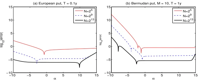
Regarding the choice of α, Lord and Kahl [27] have demonstrated recently how to approximate the optimal damping coefficient when the payoff-transform is known, which increases the numerical stability of the Carr-Madan formula. This is particularly effective for in/out-of-the-money options and options with short matu-rities. Though their rationale can to some extent be carried over to the pricing of European plain vanilla options (the difference being that now the payoff-transform is also approximated numerically), the problem becomes much more opaque when dealing with Bermudan options. To see this, note that the continuation value of the Bermudan option at the penultimate exercise date equals that of a European option. In each grid point, the European option will have a different degree of moneyness, calling for a different value ofαper grid point. The situation worsens as the number of exercise dates increases so that it is hard to say what the overall optimal value ofαwill be. What is evident from Figure 1, where we graph the error of the CONV algorithm as a function of α for a European and a Bermudan put

4

under T2-VG, is that there is a relatively large range for which the error is stable. In all numerical experiments we will set α = 0 which, at least for our examples, produces satisfactory results.

T1-GBM: S0= 100, r= 0.1, q= 0, σ= 0.25;

T2-VG: S0= 100, r= 0.1, q= 0, σ= 0.12,

θ=−0.14, ν= 0.2;

T3-CGMY: S0= 1, r= 0.1, q= 0, σ= 0,

C= 1, G= 5, M = 5, Y = 0.5; T4-CGMY: S0= 90, r= 0.06, q= 0, σ= 0

C= 0.42, G= 4.37, M = 191.2, Y = 1.0102; T5-GBM: S0= 40, r= 0.06, q= 0.04, σi= 0.2,

ρij = 0.25.

Table 1

Parameter sets in the numerical experiments

−10 −5 0 5 10 15

−10 −5 0 5 10 15

(a) European put, T = 0.1y

α

log

10

|error|

−10 −5 0 5 10 15

−10 −5 0 5 10 15

(b) Bermudan put, M = 10, T = 1y

α

log

10

|error|

N=25

N=29

N=213

N=25

N=29

N=213

Fig. 1.Error of CONV method under T2-VG and K = 110 for a European and Bermudan

put in dependence of parameterα.

5.2. European Call under GBM and VG. First of all, we evaluate the CONV method for pricing European options under VG. The parameters for the first test are from T2-VG withT = 1. Figure 2 shows that Discretisations I and II generate results of similar accuracy. What we notice from Figure 2 is that the only option with a stable convergence in Discretisation I is the at-the-money option with

K= 100. It is clear that placing the strike on they-grid in Discretisation II ensures a regular second order convergence. The results are obtained in comparable CPU time. From the error analysis in Section 4.2 it became clear that for short maturities in the VG model, the slow decay of the characteristic function (β3 = 2τ /ν) might

impair the second order convergence. To demonstrate this, we choose a call option with a maturity of 0.1 years, andK= 90. Table 2 presents the error of Discretisation II for this option in models T1-GBM and T2-VG. The convergence under GBM is clearly of a regular second order. From the error analysis we expect the convergence under VG to be of first order. Most probably the highly oscillatory integrand causes the non-smooth behaviour observed in Table 2. Note that all reference values are based on an adaptive integration of the Carr-Madan formula; all CPU times are determined after averaging the times of 1000 experiments.

In Appendix A the Greeks of the GBM call from Table 2 are computed.

8 10 12 14 16 −9

−8 −7 −6 −5 −4 −3 −2 −1 0

log 10

|error|

n, N=2n

(a) Discretisation I

K=80 K=90 K=100 K=110 K=120

8 10 12 14 16

−9 −8 −7 −6 −5 −4 −3 −2 −1 0

log 10

|error|

n, N=2n

(b) Discretisation II

K=80 K=90 K=100 K=110 K=120

Fig. 2. Convergence of the two discretisation methods for pricing European call options at

various Kunder T2-VG; left: Discretisation I, right: Discretisation II.

Table 2

CPU time, error and convergence rate for European call options under T1-GBM and T2-VG, K= 90, T = 0.1(using Discretisation II)

(N= 2n_{) GBM:V}

ref(0, S0) = 11.1352431; VG:Vref(0, S0) = 10.9937032;

n time(sec) error conv. time(sec) error conv.

7 0.0001 -2.08e-3 – 0.0002 -2.92e-4 –

8 0.0002 -5.22e-4 4.0 0.0003 -1.42e-4 2.1 9 0.0003 -1.30e-4 4.0 0.0006 -4.61e-5 3.1 10 0.0006 -3.26e-5 4.0 0.0011 -9.48e-6 4.9 11 0.0012 -8.15e-6 4.0 0.0023 -8.41e-7 11.3 12 0.0023 -2.04e-6 4.0 0.0045 8.10e-7 1.0

options under both T1-GBM and T2-VG. The reference values reported in Table 3 and 4 are found by the CONV method with 220 _{grid points.}

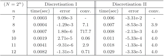
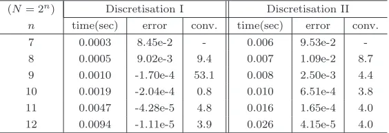
It is shown in Tables 3 and 4 that both Discretisation I and II give results of similar accuracy. Discretisation I uses somewhat less CPU time, but Discretisation II shows a regular second order convergence, enabling the use of extrapolation. The computational speed of both discretisations is highly satisfactory.

Table 3

CPU time, error and convergence rate pricing a 10-times exercisable Bermudan put under T1-GBM;K= 110, T= 1andVref(0, S0) = 11.98745352,

(N= 2n_{) Discretisation I Discretisation II}

n time(sec) error conv. time(sec) error conv.

7 0.0003 9.09e-3 - 0.006 -3.31e-2

-8 0.0004 -1.29e-3 7.1 0.007 -8.53e-3 3.9 9 0.0007 1.80e-6 717.7 0.008 -2.13e-3 4.0 10 0.0019 2.71e-5 0.06 0.011 -5.33e-4 4.0 11 0.0041 -9.31e-6 2.9 0.018 -1.33e-4 4.0 12 0.0082 -1.31e-5 0.71 0.029 -3.33e-5 4.0

opportuni-Table 4

CPU time, error and convergence rate pricing a 10-times exercisable Bermudan put under T2-VG;K= 110, T = 1with reference valueVref(0, S0) = 9.040646119.

(N= 2n_{) Discretisation I Discretisation II}

n time(sec) error conv. time(sec) error conv.

7 0.0003 8.45e-2 - 0.006 9.53e-2

-8 0.0005 9.02e-3 9.4 0.007 1.09e-2 8.7 9 0.0010 -1.70e-4 53.1 0.008 2.50e-3 4.4 10 0.0019 -2.04e-4 0.8 0.010 6.51e-4 3.8 11 0.0047 -4.28e-5 4.8 0.016 1.65e-4 4.0 12 0.0094 -1.11e-5 3.9 0.026 4.15e-5 4.0

ties, which gave robust results. In our first test we price an American put under T1-GBM. The reference value was obtained by solving the Black-Scholes PDE on a very fine grid. The performance of both approximation methods is summarised in Table 5, where ’P(N/2)’ denotes that the American option is approximated by an N/2-times exercisable Bermudan option. ’Richardson’ denotes the results obtained by the 2-times repeated Richardson extrapolation scheme. It is evident that the extrapolation-based method converges fastest and costs far less CPU time than the direct approximation approach (e.g. to reach an accuracy of 10−4_{, the extrapolation}

method is approximately 20 times faster).

In Appendix A the Greeks of the American put from Table 5 are computed.

Table 5

CPU time and errors for an American put under T1-GBM, with: K = 110, T = 1, Vref(0, S(0)) = 12.169417

(N= 2n_{) P(N/2) Richardson}

n time(sec) error conv. time(sec) error conv.

7 0.025 -6.34e-2 – 0.011 -4.88e-2 –

8 0.055 -2.34-3 2.7 0.020 8.77e-3 5.6

9 0.130 -9.49e-3 2.5 0.038 2.24e-3 3.9 10 0.346 -4.19e-3 2.3 0.078 5.53e-4 4.1 11 1.18 -1.95e-3 2.1 0.181 1.29e-4 4.3 12 3.98 -9.40e-4 2.1 0.436 2.30e-5 5.6

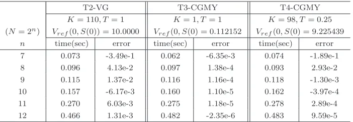
In the remaining tests we demonstrate the ability of the CONV method to price American options accurately under alternative dynamics, using the VG and both CGMY test sets. All reported reference values were generated with the CONV method on a mesh with 220 _{points and 2-times Richardson extrapolation on}

prices of American options5_.

Table 6

CPU time and errors for American puts under VG and CGMY

T2-VG T3-CGMY T4-CGMY

K= 110, T = 1 K= 1, T = 1 K= 98, T= 0.25 (N= 2n_{) V}

ref(0, S(0)) = 10.0000 Vref(0, S(0) = 0.112152 Vref(0, S(0) = 9.225439

n time(sec) error time(sec) error time(sec) error

7 0.073 -3.49e-1 0.062 -6.35e-3 0.074 -1.89e-1

8 0.096 4.13e-2 0.097 1.38e-4 0.093 2.93e-2

9 0.115 1.37e-2 0.116 1.16e-4 0.118 -1.30e-3

10 0.157 -6.17e-3 0.160 1.10e-5 0.162 -3.97e-4

11 0.270 6.03e-3 0.275 1.18e-5 0.278 2.89e-4

12 0.466 1.31e-3 0.482 -2.35e-6 0.483 9.59e-5

5.5. 4D Basket Options under GBM. The CONV method can easily be generalised to higher dimensions. The only assumption that the multi-dimensional model is required to satisfy is the independent increments assumption in (11). We do not state the multi-dimensional version of Algorithm 1 here as it is a trivial generalisation of the univariate case. Its ability to price options of a moderate di-mension is demonstrated by considering a 4-asset basket put option. Upon exercise at time ti, the payoff is:

V(ti,S(ti)) = max(

1 4

4

X

p=1

Sp(ti)−K,0). (55)

The results of pricing a European and a 10-times exercisable Bermudan put under T5-GBM are summarised in Table 7. The CPU times on the tensor-product grids are very satisfactory, especially as the results on the coarse grids obtained in only a few seconds seem to have converged to within a practical tolerance level. In order to be able to price higher-dimensional problems our future research will aim to combine the multi-dimensional CONV method with sparse grids.

Table 7

CPU time and prices for multi-asset European and 10-times exercisable Bermudan basket put options under T5-GBM,K= 40, T= 1

European 10-times exerc. Bermudan N result time (sec) result time (sec) 164

1.6428 0.02 1.7721 0.18

324

1.6537 0.51 1.7390 3.40

644

1.6539 9.5 1.7394 65.7

1284

1.6538 202.4 1.7393 1526.3

6. Conclusions. In this paper we have presented a novel FFT-based method for pricing options with early-exercise features, the CONV method. Like other FFT-based methods, it is flexible with respect to the choice of asset price process and the type of option contract, which has been demonstrated in numerical exam-ples for European, Bermudan and American options. Path-dependent exotics can in principle also be valued by a forward propagation in time, though this has not

5

been demonstrated here. The crucial assumption of the method is that the under-lying assets are driven by processes with independent increments, whose character-istic function is readily available. Though we have mainly focused on univariate exponential L´evy models, the techniques presented here certainly also extend to multivariate models, as Section 5.5 has shown. By using the FFT to calculate con-volutions we achieve a complexity ofO(M N logN), whereN is the number of grid points and M is the number of exercise opportunities of the option contract. In comparison, the QUAD method of [1] isO(M N2_{). The speed of the method may}

make it possible to calibrate models to the prices of American options, as exchange-traded options are mainly of the American type. Future research will focus on the usage of more advanced quadrature rules, combined with speeding up the method for high-dimensional problems.

Acknowledgments:The authors would like to thank Coen Leentvaar for his help in producing numbers for Table 7.

Large parts of research for this paper were performed when the first author was employed by the Modelling and Research Department at Rabobank International and the Tinbergen Institute at the Erasmus University of Rotterdam. The authors are grateful to seminar participants at Rabobank International.

REFERENCES

[1] A.D. Andricopoulos, M. Widdicks, P.W. Duck and D.P. Newton, Universal Option

Valuation Using Quadrature, J. Financial Economics, 67,3: 447-471, 2003,

[2] J. Abate and W. Whitt,The Fourier-series method for inverting transforms of probability

distributions.Queueing Systems, 10: 5–88, 1992.

[3] A. Almendral and C.W. Oosterlee, Highly Accurate Evaluation of European and

Ameri-can Options Under the Variance Gamma Process.J. Comp. Finance10(1): 21-42, 2006.

[4] A. Almendral and C.W. Oosterlee, Accurate Evaluation of European and American

Options Under the CGMY Process.,SIAM J. Sci. Comput.29: 93-117, 2007.

[5] S. I. Boyarchenko and S. Z. Levendorski˘ı,Non-Gaussian Merton-Black-Scholes theory,

vol. 9 of Advanced Series on Statistical Science & Appl. Probability, World Scientific Publishing Co. Inc., River Edge, NJ, 2002.

[6] M. Broadie and Y. Yamamoto,A double-exponential Fast Gauss transform algorithm for

pricing discrete path-dependent options.Operations Research 53(5): 764–779, 2005

[7] P. P. Carr, H. Geman, D. B. Madan, and M. Yor,The fine structure of asset returns:

An empirical investigation, J. of Business, 75, 305–332, 2002.

[8] P. P. Carr and D. B. Madan, Option valuation using the Fast Fourier Transform, J.

Comp. Finance, 2: 61–73, 1999.

[9] P. P. Carr, D. B. Madan, and E. C. Chang,The Variance Gamma process and option

pricing, European Finance Review, 2: 79–105, 1998.

[10] C-C Chang, S-L Chung and R.C. Stapleton,Richardson extrapolation technique for

pric-ing American-style optionsProc. of 2001 Taiwanese Financial Association, Tamkang University Taipei, June 2001. Available at

http://papers.ssrn.com/sol3/papers.cfm?abstract_id=313962.

[11] R. Cont and P. Tankov,Financial modelling with jump processes, Chapman & Hall, Boca

Raton, FL, 2004.

[12] H Dubner and J. Abate,Numerical inversion of Laplace transforms by relating them to

the finite Fourier cosine transform.Journal of the ACM 15(1): 115–123, 1998.

[13] D. Duffie, J. Pan and K. Singleton, Transform analysis and asset pricing for affine

jump-diffusions.Econometrica 68: 1343–1376, 2000.

[14] G. Fan and G.H. Liu,Fast Fourier Transform for discontinuous functions,IEEE Trans.

Antennas and Propagation 52(2): 461-465, 2004.

[15] R. Geske, H. Johnson,The American put valued analyticallyJ. of Finance 39: 1511-1542,

1984.

[16] J. Gil-Pelaez,Note on the inverse theorem.Biometrika 37: 481-482, 1951.

[17] J. Gurland,Inversion formulae for the distribution of ratios.Ann. of Math. Statistics 19:

228-237, 1948.

[18] S. Heston,A closed-form solution for options with stochastic volatility with applications to

bond and currency options, Rev. Financ. Stud., 6: 327–343, 1993.

[19] D. J. Higham,An Introduction to Financial Option Valuation, Cambridge University Press,

[20] A. Hirsa and D. B. Madan,Pricing American Options Under Variance Gamma, J. Comp. Finance, 7, 2004.

[21] S. Howison,A matched asymptotic expansions approach to continuity corrections for

dis-cretely sampled options. Part 2: Bermudan optionsWorking Paper, Oxford Univ., 2005.

[22] Z. Hu, J. Kerkhof, P. McCloud, and J. Wackertapp,Cutting edges using domain

inte-gration,Risk, 19(11): 95-99, 2006.

[23] P. Hunt, J. Kennedy and A.A.J. Pelsser,Markov-functional interest rate models.Finance

and Stochastics 4(4): 391-408, 2000.

[24] P. den Iseger, Numerical transform inversion using Gaussian quadratureProbab. in the

Eng. and Inform. Sciences 20(1): 1-44, 2006.

[25] R. Lee,Option Pricing by Transform Methods: Extensions, Unification, and Error Control.

J. Computational Finance,7(3): 51-86, 2004.

[26] A. LewisA simple option formula for general jump-diffusion and other exponential L´evy

processes. SSRN working paper, 2001. Available at:http//ssrn.com/abstract=282110.

[27] R. Lord and C. Kahl,Optimal Fourier inversion in semi-analytical option pricing.SSRN

working paper, 2006. Available at:http//ssrn.com/abstract=921336.

[28] A. M. Matache, P. A. Nitsche, and C. Schwab,Wavelet Galerkin pricing of American

options on L´evy driven assets, working paper, ETH, Z¨urich, 2003.

[29] S. RaibleL´evy Processes in Finance: Theory, Numerics and Emperical FactsPhD Thesis,

Inst. f¨ur Math. Stochastik, Albert-Ludwigs-Univ. Freiburg, 2000.

[30] E. Reiner,Convolution Methods for Path-Dependent Options,Financial Math. workshop,

IPAM UCLA, Jan. 2001. Available through

http://www.ipam.ucla.edu/publications/fm2001/fm2001_4272.pdf.

[31] K-I SatoBasic Results on L´evy Processes, In: L´evy Processes, 3–37, Birkh¨auser Boston,

Boston MA, 2001.

[32] C. O’Sullivan,Path Dependent Option Pricing under Levy Processes EFA 2005 Moscow

Meetings Paper, Available at SSRN: http://ssrn.com/abstract=673424, Febr. 2005.

[33] I. Wang, J.W. Wan and P. Forsyth,Robust numerical valuation of European and

Amer-ican options under the CGMY process.Techn. Report U. Waterloo, Canada, 2006.

[34] P. Wilmott, J. Dewynne, and S. Howison,Option pricing, Oxford: Financial Press, 1993.

Appendix A. The Hedge Parameters. Here, we present the CONV formulae for two important hedge parameters ∆ and Γ, defined as,

∆ = ∂V

∂S =

1

S ∂V

∂x, Γ = ∂2_V

∂S2 =

1

S2

−∂V

∂x + ∂2_V

∂x2

. (56)

As it is relatively easy to derive the corresponding CONV formulae, we merely present them here. For notational convenience we define:

F {eαxV(t0, x)}=e−r∆tA(u), (57)

whereA(u) =F {eαy_V(t

1, y)} ·φ(−u+iα), and we assumet1>0. We now obtain

the CONV formula for ∆, as

∆ = e

−αx_e−r∆t

S

h

F−1{−iuA(u)} −αF−1{A(u)}i, (58)

and for Γ:

Γ = e

−αx_e−r∆t

S2

h

F−1{(−iu)2A(u)} −(1 + 2α)F−1{−iuA(u)}

+α(α+ 1)F−1_{A(u)}i_{. (59)}

Note that the only additional calculations occur at the final step of the CONV algorithm, where we calculate the value of the option given the continuation and exercise values at time t1. Since differentiation is exact in Fourier space the rate of

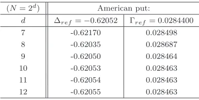
option are analytic solutions, for the American call these were found by numerically solving the Black-Scholes PDE on a very fine grid. Note that the delta and gamma of the American put converge to a slightly different value - this is due to our ap-proximation of the American option via 2 Richardson extrapolations on 128-, 64-and 32-times exercisable Bermudans. If we would increase the number of exercise opportunities of the Bermudan options the delta and gamma would, at the cost of a longer computation time, converge to their true values.

Table 8

Accuracy of hedge parameters for a European call under T1-GBM;K= 110, T= 0.1

(N= 2d_{) European call}

∆ref = 0.933029 Γref= 0.01641389

d ∆ error conv. Γ error conv.

7 -3.75e-4 – 3.79e-5 –

8 -9.37e-5 4.0 9.43e-6 4.0

9 -2.34e-5 4.0 2.35e-6 4.0

10 -5.86e-6 4.0 5.88e-7 4.0

11 -1.46e-6 4.0 1.47e-7 4.0

12 -3.66e-7 4.0 3.68e-8 4.0

Table 9

Values of hedge parameters for an American put under T1-GBM;K= 110, T= 0.1

(N= 2d_{) American put:}

d ∆ref=−0.62052 Γref= 0.0284400

7 -0.62170 0.028498

8 -0.62035 0.028687

9 -0.62050 0.028464

10 -0.62053 0.028463

11 -0.62054 0.028463

12 -0.62055 0.028463

Appendix B. Error Analysis of the Trapezoidal Rule.

Suppose we are integratingf ∈C∞ _{over an interval [a, b]. The discretisation}

error induced by approximating this integral with the trapezoidal rule follows from the Euler-Maclaurin summation formula:

Z b a

f(x)dx−T(a, b, f,∆x) =

∞

X

j=1

(∆x)2j B2j (2j)!

f(2j−1)(b)−f(2j−1)(a), (60)

whereBj is thej-th Bernoulli number andT(a, b, f,∆x) is the trapezoidal sum:

T(a, b, f,∆x) = ∆x{

N_X−1

j=1

f(xj)−

1

2(f(a) +f(b))}, (61)

with ∆x= (b−a)/(N−1) andxj=a+j∆x. From (60) it is clear that if the value

of the first derivative is not the same in a and b, the trapezoidal rule is of order 1/N2_.

The trapezoidal rule can obviously also be applied to functions that are piece-wise continuously differentiable. The convergence may however be less stable if we do not know the exact location of the discontinuities. To see this, suppose thatf

can be written as:

f(x) =

g(x) x≤z

Further, we define the following points:

ℓ= max{j|xj≤z, j= 0, . . . , N−1}, (63)

so that the interval [xℓ, xℓ+1] containsz. Placing the discontinuity on the grid would

result in the same order of convergence as the trapezoidal rule itself: Z b

a

f(x)dx≈T(a, xℓ, g,∆x) +T(xℓ+1, b, h,∆x) +

1

2(z−xℓ)(g(xℓ) +g(z)) + 1

2(xℓ+1−z)(h(z) +h(xℓ+1)). (64) A straightforward application of the trapezoidal rule would lead to T(a, b, f,∆x). The difference with (64) is:

1

2∆xg(xℓ) + 1

2∆xh(xℓ+1)− 1

2(z−xℓ)(g(xℓ) +g(z))− 1

2(xℓ+1−z)(h(z) +h(xℓ+1)). Expanding bothg andharound the point of discontinuityzyields:

1

2(xℓ+1+xℓ−2z)(g(z)−h(z)) + 1

2(xℓ+1−z)(z−xℓ)(g

(1)_(z)−h(1)_{(z)) +}

1

2(xℓ+1−z)

∞

X

j=1

1

j!g

(j)_{(z) +}1

2(z−xℓ)

j_h(j)_(z).

Iff is continuous, but the first derivatives ofg andhdo not match atz, the order of convergence is still 1/N2 _{since (x}

ℓ+1−z)(z−xℓ)≤ (∆x)2. It is clear that as

N changes, the ratio of (xℓ+1−z)(z−xℓ) to (∆x)2 may vary strongly, leading to

non-smooth convergence. If f is discontinuous, i.e., if the values of g and hin z

disagree, the order of convergence is of O(1/N).

Now suppose that we have computedgandhat grid pointsxj, j= 0, . . . , N−1.

We know that g(z) =h(z), though we do not know the exact location ofz. All we know is that it is contained in [xℓ, xℓ+1]. This is a situation we encounter in the

pricing of Bermudan options, as outlined in Section 4.4. If we proceed to integrate

f on this grid, we will not obtain smooth convergence. A simple approximation of the discontinuity can however be found by assuming a linear relationship between

xandg(x)−h(x). This leads to

z≈ xℓ+1(g(xℓ−h(xℓ))−xℓ(g(xℓ+1)−h(xℓ+1)) (g(xℓ−h(xℓ))−(g(xℓ+1)−h(xℓ+1))

+O ∆x2, (65)

where the error estimate follows from linear interpolation. Now suppose that we recalculate g and h such that either Xℓ or xℓ+1 coincide with this approximation

ofz, and redo the numerical integration. It is easy to see that smooth convergence will be restored, as the combination of the error term in(65) to the error term in (64) will be of O ∆x3_{. Note that if we use higher-order Newton-Cˆotes rules, a}