An Efficient Image Retrieval Technique using Shape
Context Feature
Neha Bhuptani
Computer EngineeringDept.Sardar Vallabhbhai Patel Institute of technology,
Vasad,Gujarat,India
Bijal Talati
HOD, Computer EngineeringDept., Sardar Vallabhbhai Patel
Institute of technology, Vasad,Gujarat,India
ABSTRACT
Increasing demands for image retrieval in field such as health informatics, biometrics, and crime prevention has forced developers to explore ways to manage and retrieve images more efficiently. An automated way to retrieve images based on the content or features of the images itself is provided by CBIR. Shape is one of key visual features used by human for distinguishing visual data along with other features of color and texture. Therefore, this work investigates one of the shape representation method shape context which helps in efficient CBIR.
The main aim of this research is to look for and develop promising shape descriptor(s) which was found to be Shape Context for image retrieval and also to improve efficiency. The Shape context descriptor is contour based which focuses on irregular shapes. The time consuming step of shape context matching is reduced in this work up to approx. 48% on an average. The proposed work reduces the computational complexity maintaining its overall accuracy.
General Terms
Feature Extraction, Image processing, Image retrieval.
Keywords
Shape Context, Content based image retrieval, Improved shape context, Contour based methods, Object recognition.
1.
INTRODUCTION
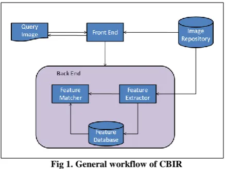
One of the challenging tasks is searching of images automatically based on its content. This field has gained attention due to its wide applications like hospitals, commerce, academics, crime prevention, and video surveillance. Generally, the problem with this task is that the irrelevant images are also retrieved. Content Based Image Retrieval or CBIR is the retrieval of these images based on visual features such as shape, colour and texture. It is considered to be a complement to the traditional textual indexing method. CBIR follows two steps that include Feature Extraction and Image Matching (or feature matching). The process of extracting features of an image to an apparent extent is termed as Feature Extraction. This extraction process is performed on both query images and images in the database. Image matching involves using the features of both images and comparing them to search for similar features of the images in the database. This whole process is explained in Fig. 1 as shown below. The front end takes an input image and passes it to back end which in turn extracts the feature and matches it with features in the feature database. The back end already maintains the feature database by extracting features from the images in repository. The matching results is passed
[image:1.595.315.535.265.430.2]to the front end and the resultant images are retrieved from the image repository.
Fig 1. General workflow of CBIR
Shape is one of the most important feature and effective due to its relevance to human perception. Shape includes the geometric information that remains integral even if rotation, scale and location effects are applied to the object [2]. Hence, shape descriptors are important. Efficient shape representation must fulfil some requisites like translation invariance, rotation invariance, scale invariance, and indentifiability, noise resistant and reliable [1]. The shape descriptor is evaluated by the requisites that it fulfils.
Shape description methods can be categorized in two ways: Contour based and Region based proposed by MPEG7. In each class, they are further classified into structural methods and global methods. This division is based on whether the shape is represented by sections or primitives or it is represented as a whole. Contour based techniques exploit the contour information. And further contour based Global methods take contour as whole into consideration while the local methods breaks the contour into small parts called primitives. The complete review of all the methods that fall under these categories is given in [4]. Also different combinations of these methods are tried and worked for image retrieval like combining chain code and fourier descriptor [6], and combining multiple simple shape descriptors [8], combining Zernike moments and shape context with the help of neuro-fuzzy classifier [9].
improvement is made in it to reduce the computational cost by maintaining its shape retrieval effectiveness.
2.
SHAPE CONTEXT AND RELATED
WORK
In [5], Belongie et al. describes the shape contexts descriptor. It indicates the coarse distribution of the rest of the shape with respect to a given point on the shape. A shape context is nothing but a histogram which displays the frequency of sample points along with their orientation and distance with respect to a reference point.
The shape context descriptor can be given by [5]:
As discussed in [1], Fig 2 [6] gives the basic idea of shape contexts. The random sample points of the two shapes are taken and shown in the Fig. 2(a) and (b). The log polar histogram is created for calculating shape context. It is shown in Fig. 2(c).
In the figure shown, one can see that, θ, the degree of the orientation, is divided into 12 bins and log r, the distance, is divided into 5 bins. In Fig. 2(d)(e)(f) shape contexts are shown (histograms) with respect to the reference points marked by ○, ◊, Δ respectively. In Fig. 2(d)(e)(f), a dark block represents the large value in that bin.
[image:2.595.320.535.79.241.2]It can be seen that the shape contexts of Fig.2 (d) and Fig. 2(e) are similar, because both figures stand for the fairly similar points on two shapes. The corresponding points on the two shapes will have similar shape context due to this similarity in shape. So, one can see that shape context is dependent on the size and orientation of shape.
Fig 2. Shape context diagram
Consider a point pi on the first shape P and a point qjon the
second shape Q. The cost of matching between two points pi
and qjis denoted by C ( pi,qj)and is computed by using the χ 2
test statistic as given in [8] is formulated in Eq. (2) which is given as follows:
The numbers of bins are decided such that they are uniform in log polar space. The shape context descriptor has the invariance properties like translation, scaling, rotation.
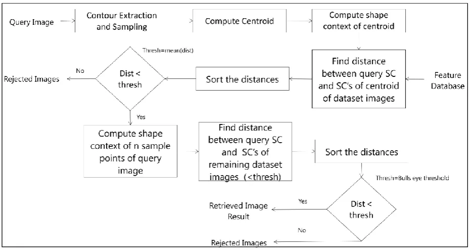
Fig 3. Proposed Work
The most expensive step in above mentioned approach is calculating the cost matrix for matching the two shapes. This leads to a disadvantage of expensive computation. As a result it could not be applied to huge database. So many variations
[image:2.595.65.531.451.698.2]In [10], SIFT descriptor is combined with the shape context descriptor to combine the effect of local feature points and global sample points of shape context for leaf image classification. But this does not solve the problem of high computation in shape context.
In [7], the shape contexts (histograms) are rearranged into a 1D shape context vectors. As a result, the expensive step of point to point matching is reduced to matching of single dimension vectors.
3.
PROPOSED METHOD
In this paper, a new algorithm has been proposed for shape context where it is divided into two stages. The first stage is preliminary stage which helps in reducing search area for the next stage of matching. As a result efficiency of an algorithm increases reducing computational complexity.The overall workflow can be seen in Fig. 3.
3.1
Pre-processing and Sampling
To get the experimental results, Matlab was used as its one of the dominant tool for image processing. In first stage, image is taken as an input and preprocessing is done if necessary. It is required to get a proper contour of an object from an image. In preprocessing, filtering is performed on an image to remove the noise. The filter used is median filter so as to preserve edges. Next, perform morphological operations to
smooth the boundary of an object. Now subtract the morphed image from an original image to get a proper contour. As a result smooth boundary is obtained. After the segmented object is obtained, apply boundary tracing algorithm using 8-connectivity. As a result contour is extracted from an object.
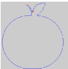
After preprocessing and contour extraction is performed, sampling is done. That is downsample the contour to some particular number of sample points. Let’s say P=200. These sample points are equidistant to each other. All these operations are shown in Fig. 2.
3.2
Preliminary Filtering Stage
Centroid is one of the global parameter of the shape. It captures the global information of a shape Centroid can be defined by equation [3]:
This centroid can be incorporated with the concept of shape Context. Shape context is calculated by keeping centroid as a respective point.
[image:3.595.324.466.359.504.2]Calculate the angular distances and radial distances between sample points extracted from contour and centroid. Using these distances calculate the shape context.
Fig 4. Input Apple image Fig 5. Extracted Boundary
The shape context of centroid will have one dimensional vector. As a result the feature vector generated is of very low dimension. Now this shape context of centroid of query image is matched with the shape context of the centroid of the images in the database. The distance between two centroidal shape contexts is calculated using chi square distance which is defined as given in equation (1).
The distance calculated is compared with the threshold as shown in Fig. 3. The images having distance less than threshold are passed for further investigation. Reject the remaining images. This shows that the number of images for further investigation will be reduced to a great extent.
3.3
Final Stage
After filtering is performed, the candidate images have reduced to a great extent and these images are matched by their original shape context feature vector. Hence, the shape context descriptor is created for P sample points. This leads to feature vector of 2 D. The dimension of this feature is comparatively very high than the centroidal feature vector. These feature vectors are matched with each other. This leads to a very time consuming step as explained. So the reduction in candidate images will reduce the time and improve performance.
After the distances are calculated, they are sorted in increasing order. And bull’s eye score is used to retrieve the relevant images and measure the accuracy of the retrieval performance. Suppose we have p positive examples for a given query in the database, the Bull’s eye measure is computed as the amount of correctly retrieved items in the first 2 × p results. So the images are retrieved through the use of bulls eye measure [11].
4.
EXPERIMENTAL RESULTS
The inclusion of the centroid filtering helps in reducing the no of images to be matched in the crucial step. As a result computational complexity reduces and performance increases.
4.1
Dataset and Performance Evaluation
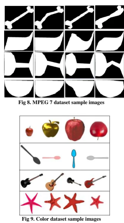
To derive the experimental results, the use of two datasets is done. One is the widely used MPEG 7 dataset containing 1400 binary images of 70 categories [12]. Each category contains 20 images. Some sample images of this dataset is shown in Fig. 8. Another one is the color image dataset created from the images taken from the web. It contains 150 images of 15 categories. Each category contains 10 images. Sample images of this dataset are shown in Fig. 9. To evaluate performance, Bulls eye score is used. In MPEG 7 dataset, each category contains 20 images. So, top 40 images from the increasing order of distances are retrieved to measure accuracy. Same way, color image dataset contains 10 images in each category. So, top 20 images are retrieved to measure accuracy.The experiments performed here takes P= 200 sample points from the images. The crucial computing step in this work is matching of the histograms i.e calculating the distance between the query image and the dataset images which is most time consuming due to the size of the histograms. There occurs a need to match (no of sample points*no of bins) size histogram of each image.
[image:4.595.325.534.64.440.2]The computational complexity can be measured as shown here. Let N be the number of images in the dataset repository. Let P be the number of sample points extracted from the image. Let R be the number of radial bins and A be the number of angular bins.
Fig 8. MPEG 7 dataset sample images
Fig 9. Color dataset sample images
Therefore, total number of bins B= R*A. In this experiment, R=5, and A=15 is taken.
Total number of computations required for histogram matching in an original shape context method without filtering will be:
Where (P*B) is the size of the feature vector containing P sample points.
While to find total number computations required for histogram matching by a proposed work, first find the computations required for centroidal histogram matching and then find computations required for left over candidate histogram matching. For centroidal histogram matching computations required will be:
Where (1*B) is size of feature vector containing shape context of centroid.
After filtering, the image candidates to be matched reduce by approx. 48 % in the database that are used. So matching reduces to 48% size. Hence, computations required for histogram matching of remaining candidates (52%) by original shape context computation will be:
[image:5.595.314.554.78.260.2]
Here, time consuming computation has been reduced by 48%. The addition of computations by centroidal histogram matching results in very little computational cost because of the smaller size of the feature vector. As a result, the overall computational cost reduces and thereby increases the performance.
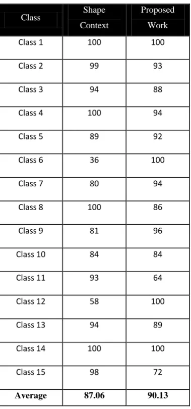
Table 1. Color Dataset Analysis
Class Shape
Context
Proposed
Work
Class 1 100 100
Class 2 99 93
Class 3 94 88
Class 4 100 94
Class 5 89 92
Class 6 36 100
Class 7 80 94
Class 8 100 86
Class 9 81 96
Class 10 84 84
Class 11 93 64
Class 12 58 100
Class 13 94 89
Class 14 100 100
Class 15 98 72
Average 87.06 90.13
4.2
Results
The experimental results for dataset of color images in detail are shown in table 1. The comparison is made with the shape context and proposed work. It is also shown in Figure 10 the comparison is shown graphically. After the experiments were performed, the results derived are shown in table 2. The comparison between the original shape context method and the proposed work is shown. The bulls eye accuracy of both methods is shown on two datasets used. Last column indicates the % reduction in dataset images for further investigation after the completion of first stage of filtering. It can be seen from the table that the overall bull’s eye accuracy of the retrieval is preserved by reducing the computational complexity. Instead the overall accuracy is increased by average 2%.
Fig 10. Color dataset sample images
Table 2. Overall Analysis
Dataset
Shape Context
(Bull’s eye Accuracy)
Proposed Work
(Bull’s eye Accuracy)
% Reduction of dataset in Final stage
MPEG7
Binary dataset 79.19 80.50 47.2636
Color Images
Dataset 87.06 90.13 45.3867
5.
CONCLUSION AND FUTURE WORK
The crucial computing step in this work is matching of the histograms i.e calculating the distance between the query image and the dataset images which is most time consuming due to the size of the histograms. There occurs a need to match (no of sample points*no of bins) size histogram of each image. So, in this paper, a proposed method is implemented where a centroid concept is incorporated with shape context to perform preliminary filtering. This results in improvement in overall accuracy as well by reducing the computational cost. We can see that computational overhead reduces by approx. 48% after filtering. The first step of preliminary filtering has negligible overhead compared to actual overhead. So it can be ignored. This work helps in reducing computation overhead while maintaining accuracy.
The proposed method takes the tradeoff into consideration. The more you increase the sample points, the more accuracy is obtained but with the increase in the computational overhead. So, this filtering helps in reducing this overhead, when more accuracy is required. Also, this proposed method will be very helpful when the size of the image repository will be very high. As, in that case, the reduction in computational cost will be very good. Still this proposed work can be improved by adding more parameters to its filtering stage. So, the proposed work should be further investigated for refinement.
6.
REFERENCES
[1] Neha Bhuptani and Bjial Talati. Article: Variations in Shape Context Descriptor: A Survey. International Journal of Computer Applications 90(12):29-33, March 2014.
[image:5.595.73.263.186.592.2][3] Yang, Mingqiang, KidiyoKpalma, and Joseph Ronsin.
"A survey of shape feature extraction
techniques." Pattern recognition (2008): 43-90.
[4] Zhang, Dengsheng, and Guojun Lu. "Review of shape representation and description techniques." Pattern recognition 37, no. 1 (2004): 1-19.
[5] Belongie, Serge, Jitendra Malik, and Jan Puzicha. "Shape
matching and object recognition using shape
contexts." Pattern Analysis and Machine Intelligence, IEEE Transactions on 24, no. 4 (2002): 509-522. [6] Geevar, C. Zacharias, and P. Sojan Lal. "Combining
Chain-Code and Fourier Descriptors for Fingerprint
Matching." Advances in Computing and
Communications. Springer Berlin Heidelberg, 2011. 460-468.
[7] Schlosser S., and Beichel, R. “Fast Shape Retrieval Based on Shape Contexts” In Image and Signal Processing and Analysis, 2009. ISPA 2009.
[8] Sarfraz, Muhammad, and A. Ridha. "Content-based
image retrieval using multiple shape
descriptors." Computer Systems and Applications, 2007. AICCSA'07. IEEE/ACS International Conference on. IEEE, 2007.
[9] Lopez, Annet Deenu, Eldho S. Kollialil, and K. Gopika Gopan. "Adaptive Neuro-fuzzy Classifier for Weapon Detection in X-Ray Images of Luggage Using Zernike Moments and Shape Context Descriptor." Advances in Computing and Communications (ICACC), 2013 Third International Conference on. IEEE, 2013.
[10] Wang, Zhiyong, et al. "Leaf Image Classification with Shape Context and SIFT Descriptors." Digital Image Computing Techniques and Applications (DICTA), 2011 International Conference on. IEEE, 2011.
[11] Rusiñol, Marçal, and JosepLladós. "Efficient logo retrieval through hashing shape context descriptors." In Proceedings of the 9th IAPR International Workshop on Document Analysis Systems, pp. 215-222. ACM, 2010.
[12] Image dataset of MPEG7 [Online]