Simulink Implementation for Improvement of Vehicle Directional Control using Relay Experiment Method

Simulink Implementation for Improvement of Vehicle

Directional Control using Relay Experiment Method

B. Srinivas B. Lavanya P. Surya Prasad

(Assistant Professor) (Assistant Professor) (Associate Professor)

Dept. Electronics and Communication Engineering,

M.V.G.R.College of Engineering, Vizianagaram, Andhra Pradesh, India

ABSTRACT

The objective of this paper is to provide directional control during handling maneuvers and effective isolation of passengers or pay load from road disturbances. Active suspension system is considered to be a way of increasing the freedom that one has to specify independently the characteristics of load carrying, handling and ride quality. In this paper, a quarter bus suspension system is simulated and the behaviour of the system has been analyzed for disturbances. A PID controller is designed by the method of relay experiment and is considered for control of the Quarter bus suspension system.

General Terms

Keywords

Vehicle Directional control, PID tuning, Riding comfort, Relay experiment method.

1.

INTRODUCTION

Passive suspension system is the most popular system used in commercial trucks because of its simplicity and cost compared to other types of suspension system. An important aspect of passive suspension system in vehicle is the cushion of the seat, which is in direct contact with the human operator and transmits the characteristics of the suspension system to the human. However, since the cushion also has stiffness and damping characteristics, it also acts as a suspension, making it a two-degree of freedom system, and enables a potential increase in suspension system.

Traditionally, automotive suspension designs have been a compromise among the three conflicting criteria of road holding, load carrying and passenger comfort. The suspension system must support the vehicle, provide directional control during handling maneuvers and provide effective isolation of passengers/payload from road disturbances. Good ride comfort requires a soft suspension, whereas insensitivity to applied loads requires stiff suspension. Good handling requires a suspension setting somewhere between the two.

1.1 PID Controller

A proportional-integral-derivative controller (PID controller) is a generic control loop feedback mechanism (controller) widely used in industrial control systems[5]. A PID controller attempts to correct the error between a measured process variable and a desired set point by calculating and then outputting a corrective action that can adjust the process accordingly and rapidly, to keep the error minimal[8].

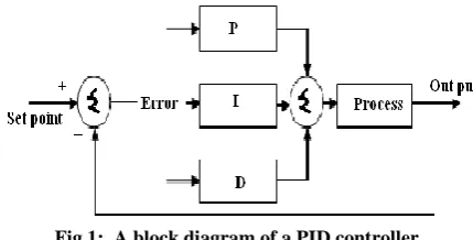
Fig 1: A block diagram of a PID controller.

The PID controller calculation (algorithm) involves three separate parameters; the proportional, the integral and derivative values. The proportional value determines the reaction to the current error, the integral value determines the reaction based on the sum of recent errors, and the derivative value determines the reaction based on the rate at which the error has been changing [1] as shown in Table 1. The weighted sum of these three actions is used to adjust the process via a control element such as the position of a control valve or the power supply of a heating element.

TABLE IResponse of Proportional, Integral and Derivative Controller

Close d loop Respo

nse

Rise Time

overshoot Settling time

Steady state error

KP Decrease Increase No change

Decrease

KI Decrease Increase Increase Eliminate

KD No

change

Decrease Decrease No change

) ( )

( )

( )

( )

(

0

t dt de k d t e k t e k t MV t

u

t

d i

p 





 

1.2 Relay Experiment

The relay is an ON-OFF control device, and this is the experimental core of the new controller unit. The characteristic of the relay is shown in fig2.

Fig 2: The ON-OFF relay characteristics

INPUT:

Error signal from comparator e(t) OUTPUT:

If e(t)<0 then u(t)=-M If e(t)>=0 then u(t)=+M

These new process controller devices typically have an auto tune button marked A or T (A for Auto tune or T for Tune). When pressed, an automatic procedure starts whereby the closed- loop controller is switched to the ON-OFF relay and system oscillation is set up. This is monitored at the error signal e(t) and used by a signal processing unit to find the ultimate gain Ku and ultimate period, Pu. This data is used in

rule base to compute PID parameters. Finally, the parameters are passed to the actual PID controller algorithm and control switched from the ON-OFF relay back to the PID controller. This completes the process of automated PID controller tuning.

Fig 3: the relay feedback loop setup

This procedure sounds remarkably like the sustained oscillation method in that the relay experiment finds the process’s ultimate data, Ku, and Pu(from the fig4) through the

use of a oscillation. Indeed this to be case, since the relay sets up a stable oscillation at the phase crossover reference, wpco.

Technically this oscillation a limit cycle. Consider the system depicted in Fig3. Assuming there is a limit cycle with period Pu, so the relay output is a periodically symmetric wave. 

The significant and important difference from the sustained oscillation experiment is that the relay experiment produces a self-generated and stable oscillation; so that the closed loop system does not have to be driven to the verge of instability. The role of the signal processing component of the controller unit is to find the ultimate period, Pu, and to measure the

amplitude of the oscillation, which is called Aosc. The ultimate

gain Ku is s found out using a very simple formula

OSC

A M u

k



_

Where M is the height of the ON-OFF relay controller characteristic.

The immediate aspect of the relay experiment which makes it such an attractive solution to the automated PID problem is its simplicity. It is easy to implement, and the computations

needed to find Ku and Pu are simple in form. Some added

bonus can also be identified: for example the height of the relay M can be used to control the size of the process output oscillation, thereby reducing the disturbances to production operations. Relay experiment is a one-off procedure, so that the necessity to conduct a repeated sequence of test experiments is avoided.

Fig 4: The output response from relay feedback

2.

MODELING FOR SUSPENSION

SYSTEM

2.1 Modeling of Quarter Bus Suspension

System

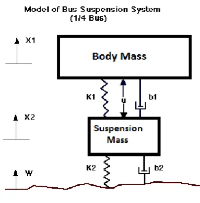
Fig 5: Quarter Bus suspension Model.

Designing an automatic suspension system for a bus turns out to be an interesting control problem. When the suspension system is designed, a 1/4 bus model (one of the four wheels)is used to simplify the problem to a one dimensional spring-damper system[1]. A diagram of this system is shown in fig 5. Consider

* Body mass (m1) = 2500 kg, * suspension mass (m2) = 320 kg,

2.2 Schematic Diagram

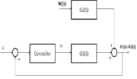
The schematic system looks as in fig 6. This concept is discussed in section E [1].

Fig 6: Schematic Model of the Bus Suspension System

2.3 Design requirements

A good bus suspension system should have satisfactory road holding ability, while still providing comfort when riding over bumps and holes in the road. When the bus is experiencing any road disturbance (i.e. pot holes, cracks, and uneven pavement),the bus body should not have large oscillations, and the oscillations should dissipate quickly. Since the distance X1-W is very difficult to measure, and the deformation of the tire (X2-W) is negligible, the distance X1-X2 will useinstead of X1-W as the output in this work. Keep in mind that this is estimation.

The road disturbance (W) in this problem will be simulated by a step input. This step could represent the bus coming out of a pothole. A feedback controller has to be designed so that the output (X1-X2) has an overshoot less than 5% and a settling time shorter than 5 seconds. For example, when the bus runs onto a 10 cm high step, the bus body will oscillate within a range of +/- 5 mm and return to a smooth ride within 5 seconds [1].

2.4 Equations of motion

The dynamic equations of the bus suspension system were obtained by Newton’s second law of motion, and the equations are presented below:

2.5 Transfer Function Equation

Assume that all of the initial conditions are zeroes, so these equations represent the situation when the bus's wheel goes up a bump. The dynamic equations above can be expressed in the form of transfer functions by taking Laplace Transform of the above equations. The derivation from above equations of the Transfer Functions G1(s) and G2(s) of output,X1-X2, and two inputs, U and W, are as follows.

or

Find the inverse of matrix A and then multiple with inputs U(s)and W(s) on the right hand side as the following:

When input U(s) only is considered, W(s) is set to 0. Thus the transfer function G1(s) is obtained as the following:

When input W(s) is only considered, U(s) is set to 0. Thus the transfer function G2(s) is obtained as the following:

Also the above equations can be expressed and derived in state-space form. Even though this approach express the first two equations above in the standard form of matrix, it can simplify the transfer function without going through any algebra, because a function tf2ss can be used to transform from state-space form to transfer function form for both inputs. Using above values, the transfer functions of G1(s) and

G2(s) for a step input are obtained as follows.

G1(s) = nump/denp

2820 s^2 + 15020 s + 500000

= --- 800000 s^4 + 3.854e007 s^3 + 1.481e009 s^2 + 1.377e009 s + 4e010

G2(s) = num1/den1

-3.755e007 s^3 - 1.25e009 s^2

= --- 800000 s^4 + 3.854e007 s^3 + 1.481e009 s^2 + 1.377e009 s + 4e010

3.

CONTROLLER DESIGN

3.1 The relay experiment procedure

3.1.1 The process set up

The process must be in quiescent condition and in closed-loop operation. During the experiment no process disturbances must occur and measurement noise should be minimal. If a process disturbance occurs during the relay experiment, then it will effect fairly quickly. In some cases the oscillation becomes non-regular, and in more extreme cases the process oscillation will cease altogether. In the process controller technology, small modifications to the procedure have been introduced to mitigate the possible erroneous effects due to the presence of measurement noise. The changes have not been considered in this procedure.

For the most situations, the relay height M is selected by trial and error, but it must be selected to be sufficiently large to set up the limit cycle oscillation. The amplitude of the process oscillation Aosc can be fine-tuned by changing the size of M.

Fig 7: Simulink simulation for the process with Relay feedback

Apply the relay block to the process transfer function block produces appropriate oscillations to get the sustain oscillations. Then simulate the above setup the sustain oscillations are obtained, which are shown in the Fig 8.

3.1.3 Processing the data

A small pulse is used at the reference input to activate the oscillations, and the transient behaviour of the system dynamics must be allowed to settled out before attempting to process the data. The steady state portion of the response must be used for measuring the values of Pu and Aosc.

Fig 8: Output of the process with Relay feedback.

As per simulation results, from the graph The ultimate period Pu=0.99sec

Height of the ON-OFF relay M=1 Amplitude of oscillation Aosc= 3x10-5.

In real process situations the recorded traces are contaminated by noise and possible outliners. Despite these problems, the measurement should be made as best as possible. It is possible that this may require taking the means of a set of sampled measurements. The two parameters are measured:

The ultimate period Pu and the Amplitude of oscillation Aosc

as shown in above Fig 4.

3.2 Calculation of PID Parameters

When the data processing step has been completed the values of the following parameters are obtained

The recorded relay height M=1

The measurement of the ultimate period, Pu=0.99sec

The measurement of the oscillation Amplitude Aosc=3x10 -5

Ultimate gain is given by the formula Ku=4M/(πAosc)

The values for Ku and Pu are then used on a rule base to

compute an appropriate PID controller.

According to the Ziegler and Nichols method [1] [2]. Kp=0.6*Ku, Ti= 0.5*Pu, Td= 0.125*Pu. Finally the

parameters of PID controller are Kp=24771,

Ki=Kp/Ti=49542,Kd=Kp*Td=30964.

4.

SIMULATION AND RESULTS

4.1 Simulink model of process transfer

function

The process transfer function in the form, nump/denpcan be simulated as a open-loop system (without any feedback control) to control input u and its simulink model is shown in Fig 9.

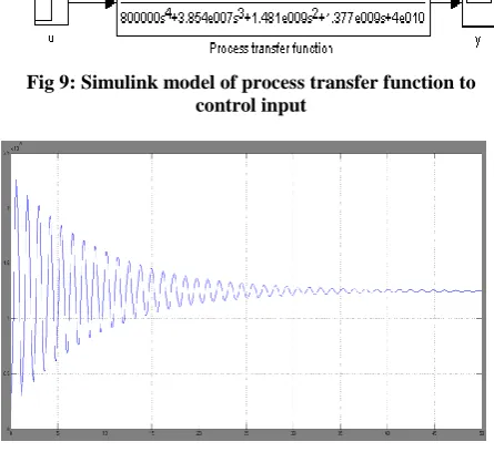
Fig 9: Simulink model of process transfer function to control input

Fig 10: Response of the process transfer function to control input.

The Fig 10 shows the open-loop response of the process transfer function for a unit step actuated force (u), and it indicates that the system is under-damped. People sitting in the bus would feel very small amount of oscillations and the steady state error is about 0.013mm. Moreover the bus takes very unacceptable long time for it to reach the steady state or the settling time is very large. The solution to this problem is to add a feedback controller into the system’s block diagrams.

Fig 11: Simulink Model for 0.1m disturbance transfer Function

Fig 12: Response of the process transfer function to 0.1m disturbance

The open-loop response of the quarter bus suspension system model for 0.1m step disturbance is observed from the Fig 12. When 0.1m step input apply to the process at 10th second, the system gets oscillations from 10th second. i.e., When the bus passes through a 0.1m high bump on the road, bus body will oscillate for an unacceptably long time (100seconds) with larger amplitude. The people sitting in the bus will not be comfortable with such an oscillations. This big overshoot and the slow settling time will cause damage to the suspension system. The solution for this problem is to add a feedback controller into the system to improve the performance.

4.2 Simulation of PID Controller

Fig 13: Simulink model for Quarter bus suspension system tuning with PID Controller.

After find out the PID controller parameters ,the values Kp, Ki

and Kd are put in the PID block, then this PID block is added

to the process. which is shown in the above Fig 13.finally run the simulink model, then the required specifications are achieved in the following graph.

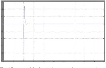
Fig 14:Response of the Quarter bus suspension system tuning with PID Controller.

According to the given 0.1m disturbance, the response of the quarter bus suspension system tuning with PID controller is as shown in the Fig 14. From this graph, the overshoot and

settling time met the requirements of the system. The overshoot is about 5%of the input’s amplitude and settling time is 5 seconds.

5.

CONCLUSION

In this paper, the transfer function of a quarter bus suspension system is obtained, simulated and the behaviour of system has been analysed for disturbances. The parameters of the PID controller are calculated and is designed by the method of relay experiment and is considered for control of the Quarter bus suspension system. The whole work is carried out in Simulink of MATLAB. The above work can also be implemented by using adaptive control algorithms so that the controller parameters can be altered automatically according to the changes in the system parameters.

6.

REFERENCES

[1] A. Karthikraja, G. Petchinathan, S. Ramesh, Stochastic Algorithm for PID Tuning of Bus Suspension System, IEEE Proc.INCACEC 2009.

[2] Kiam Ha, Chong G, Yun L (2005) PID control system analysis, design,and technology. IEEE Trans Control Syst Technol 13(4):559-576

[3] George stephanopoulous. Chemical process control: An introduction to theory and practice. Pearson education

[4] Vratislav MICHAL, Christophe PRÉMONT,Gaël PILLONET, Nacer ABOUCHI, Single Active Element PID Controllers, IEEE Circuit and Systems ISCAS, 2010.

[5] DWYER, A. Handbook of PI and PID controller tuning rules. Book, Imperial College Press, 2006.

[6] M. A. Johnson, and M. H.Moradi (Editors), PID Control, Springer-Verlag, London, 2005.

[7] M. Jamei, M. Mahfoul and D. A. Linkens, “Fuzzy Based Controller of A Nonlinear Quarter Car Suspension System, ”Student Seminar in Europe, Manchester, UK, May 20-21, 2000.

[8] Dirman Hanafi PID Controller Design for Semi-Active Car Suspension Based on Model from Intelligent System Identification, ICCEA.2010.

[9] YOU-BO WANG, XIN PENG, BEN-ZHENG WEI, A New Particle Swarm Optimization Based Auto-Tuning Of PID Controller, Machine Learning and Cybernetics, Kunming

7.

AUTHOR’S PROFILES

B. Srinivas

Received his Bachelor of Engineering in Electronics and Communication Engineering from Sir C.R.Reddy College of Engineering, Eluru, Andhra Pradesh in 2007 and received his Master of Technology in Automotive Electronics from VIT University, Vellore, Tamilnadu in 2009. He has 5 years of teaching experience and 5 international journals and conferences to his credit. Presently he is working as Assistant Professor in the department of ECE, M.V.G.R. College of Engg, Vizianagaram, Andhra Pradesh, India. His field of interest includes Control systems, Micro controllers, Electronics

B. Lavanya

Bangalore, Karnataka. Now she is pursuing Ph.D in Andhra University. she has more than 9 years of teaching experience and has 4 international journals and conferences publication. Presently she is working as Assistant Professor in the department of ECE, M.V.G.R. College of Engg, Vizianagaram, Andhra Pradesh, India. Her areas of interest are Digital electronics, circuit design.

Surya Prasad P.

Received his M.Tech. (Communication and Radar Engineering) from IIT, Delhi and B.Tech (ECE) from JNTU