Modelling and application of condition based maintenance for a two component system with stochastic and economic dependencies

M o d e lli n g a n d a p p li c a tio n of

c o n di tio n-b a s e d m a i n t e n a n c e fo r

a t w o-c o m p o n e n t s y s t e m wi t h

s t o c h a s ti c a n d e c o n o m i c

d e p e n d e n ci e s

D o, P, Ass af, R, S c a rf, PA a n d I u n g , B

h t t p :// dx. d oi.o r g / 1 0 . 1 0 1 6 /j. r e s s . 2 0 1 8 . 1 0 . 0 0 7

T i t l e

M o d elli n g a n d a p p lic a tio n of c o n di tio n-b a s e d m a i n t e n a n c e

fo r a t w o-c o m p o n e n t s y s t e m wi t h s t o c h a s ti c a n d e c o n o m i c

d e p e n d e n ci e s

A u t h o r s

D o, P, As s af, R, S c a rf, PA a n d I u n g , B

Typ e

Ar ticl e

U RL

T hi s v e r si o n is a v ail a bl e a t :

h t t p :// u sir. s alfo r d . a c . u k /i d/ e p ri n t/ 4 8 6 7 2 /

P u b l i s h e d D a t e

2 0 1 9

U S IR is a d i gi t al c oll e c ti o n of t h e r e s e a r c h o u t p u t of t h e U n iv e r si ty of S alfo r d .

W h e r e c o p y ri g h t p e r m i t s , f ull t e x t m a t e r i al h el d i n t h e r e p o si t o r y is m a d e

f r e ely a v ail a bl e o nli n e a n d c a n b e r e a d , d o w nl o a d e d a n d c o pi e d fo r n o

n-c o m m e r n-ci al p r iv a t e s t u d y o r r e s e a r n-c h p u r p o s e s . Pl e a s e n-c h e n-c k t h e m a n u s n-c ri p t

fo r a n y f u r t h e r c o p y ri g h t r e s t r i c ti o n s .

Condition-based maintenance for a two-component system

with

stochastic and economic

dependencies

Phuc Do1∗, Roy Assaf2, Phil Scarf3 and Benoit Iung1

1

Universit´e de Lorraine, Vandoeuvre-les-Nancy, 54506, France

2

Autonomous Systems and Robotics Research Centre, University of Salford, Salford, M5 4WT, UK

3

Salford Business School, University of Salford, Salford, M5 4WT, UK

Abstract

This paper develops a model of a condition-based maintenance policy for a two-component

system with both stochastic and economic dependencies. The stochastic dependency is such

that the degradation rate of each component depends not only on its own state

(degrada-tion level) but also on the state of the other component. The economic dependency is such

that combining multiple maintenance activities has lower cost than performing maintenance on

components separately. To select a component or components to be preventively maintained,

adaptive preventive maintenance and opportunistic maintenance rules are proposed. A cost

model is developed to find the optimal values of decision variables. A case study of a gearbox

system demonstrates the utility of the proposed model.

Keywords: Condition-based maintenance, maintenance optimization, two-component system,

state dependence, stochastic dependence, economic dependence.

1

Introduction

Maintenance involves preventive and corrective actions that are carried out to retain a technical

system in or restore it to an operating condition. Maintenance optimization aims to

deter-mine effective and efficient maintenance plans for each component of a system in order to meet

operator requirements for safety, reliability and value. In the literature, many policies have

been developed for the maintenance of single-component systems [8, 31]. Such maintenance

policies may be applied to multi-component systems when the dependencies between

compo-nents in these systems are neglected. However, for many technical systems it is not reasonable

to assume components are independent, and it is necessary to model component

dependen-cies. Dependencies can be classified into three main types [21, 6, 10]: (i) economic dependence,

whereby the cost of joint maintenance of a group of components does not equal the sum of individual maintenance costs for these components; (ii) structural dependence, whereby

compo-nents structurally form a part, so that maintenance of a failed component implies maintenance (at least the dismantling) of other unfailed components; (iii) stochastic dependence whereby the

state of a component influences the lifetime distribution of other components. Recently, in [16], stochastic dependencies have been categorized in three groups: (i) failure-induced damage or

failure dependence, whereby the failure of a component can lead to failure of other components; (ii) load sharing, whereby the failure of a component can increase the degradation rate of other

components; and (ii) common-mode degradation, whereby an increase in degradation of one component is associated with an increase in degradation of other components. It is important to note that a fourth type of dependence, namely resource or logistical dependence, has been also

identified in [16]. Indeed, resource dependence exists when several components are connected though a shared and limited set of spares. For example if a single repairman is responsible for

the maintenance activities of various units or systems, or if a single stock of spare parts is used

for the replacement of multiple units .

Taking into consideration dependencies between components when modelling maintenance

of multi-component systems has recently shown an increase in popularity among researchers

[4, 10, 12, 14, 21, 26]. An overview about recent advances on condition-based maintenance for

systems with multiple dependent components is given in [16]. In fact, economic dependence

has been investigated and integrated in a number of multi-component maintenance models

[10, 18, 21, 28]. However, in these works, stochastic and structural dependence are not

consid-ered. Failure dependence between components has been studied in the context of inspection by

[12] and maintenance and warranty optimization by [26, 35] for two-component systems. In the

latter, several block replacement models considering both economic and failure interaction are

proposed. Condition-based maintenance (CBM), in which the preventive maintenance decision

is based on the observed system condition, has been introduced and has become an important

developed for two-component systems, see for example [2, 5, 18]. However, in such maintenance

models, again only economic dependence is considered. Recently, a new type of stochastic

dependence, called degradation interaction or state dependence, whereby the degradation evo-lution of a component depends on both its degradation level and that of other components,

has been introduced in [3, 4] for prognostics of system lifetime, and in [23] for maintenance optimization. However, this latter work considers neither economic dependence nor intrinsic

state dependence (whereby state evolution of a component depends on its own state). Thus,

there is a need to consider multiple dependencies in CBM maintenance. With this in mind, this

paper develops a model of condition-based maintenance that takes account of both stochastic

dependence (intrinsic and extrinsic), through a model of rate-state interactions, and economic

dependence that is natural when there is rate-state interaction.

In particular, we propose a CBM model for a two-component system with rate-state

inter-action, whereby the degradation rate of each component depends not only on its own state but

also on the state (degradation level) of the other component. This dependence phenomenon can

be found in a number of industrial systems, e.g. the state (quality) of oil may directly impact

the degradation process of the crank and vice versa, wear on a pulley may impact the rate of

wear of a belt and vice versa (Mark Maher, 2015, “Below the belt”, Maintenance Engineering,

July/August, p.17), and likewise for chains and gears. In our model, we suppose that

inspec-tions occur at regular time intervals and identify the state of each component. Maintenance

actions are then (optimally) planned based on the current, inspected state of the components,

and broadly corresponds to a choice of: do nothing; replace component 1 and not component 2;

replace component 2 and not component 1; or replace both. An interesting consequence of the

rate-state interaction that we study is that when one component is replaced but not the other,

obviously the system is not perfectly maintained (i.e. it is not renewed), but more interestingly

the new component will deteriorate at a different rate to that when the system was new, because

the degradation rate of the new component depends on the state of the old component. This

partial replacement, or imperfect maintenance, of the system is then an imperfect “repair” that

considers imperfect repair in a different way to the existing approaches in the literature, in which

age/hazard reduction models predominate [8, 33, 34]. It is important to note that when

con-sidering state dependence between components, existing CBM models may lead to sub-optimal

policies. This is because degradation modelling has a significant impact on the determination

of optimal maintenance policy in CBM and, in these existing CBM models, state dependence is

a CBM policy in which adaptive preventive maintenance and opportunistic maintenance rules

select a component or group of components to be maintained, and in so doing to open a new

strand of thinking in the modelling of imperfect maintenance. A cost model is developed to find

the optimal maintenance policy. We argue that ignoring stochastic dependence will lead to a

maintenance policy that is cost-inefficient. Thus, in our view, our model makes a contribution

to the literature that will not only lead to further developments in maintenance optimization

for systems with stochastic dependence but also be useful for practical application.

The paper is organized as follows. In the next section, we describe the model of the system

and its dependencies. Both state and economic dependencies are herein investigated. Section 3

describes the proposed maintenance policy and the optimization process. To demonstrate the

utility of the proposed maintenance policy, a case study of a gearbox system is introduced in

Section 4. In the results we include sensitivity analyses. In the final section we presents our

conclusions and discuss the managerial implications of the work.

Notation

a cost-saving factor for joint replacement (when components 1 and 2 are replaced together)

b duration-saving factor for joint replacement

C∞ long-run expected maintenance cost per time unit (cost-rate) CS−,− cost-saving of joint replacement

CI cost of an inspection

Ci

p,Cci cost of preventive and corrective replacement of component irespectively

cd downtime cost-rate of the system

di duration of a replacement for component i

Ti the time of the ith inspection of the system

∆T inter-inspection interval

xi_Tk state (degradation level) of component iat timeTk

Li _{failure threshold of component i}

mi

p, mio preventive and opportunistic maintenance thresholds for componenti

2

System description and dependency modelling

Consider a series system with two dependent components. When one or both components fail

the system fails. Each component iis subject to a continuous accumulation of degradation in

time that is assumed to be described by a scalar random variableXi

t. Componentiis considered

as failed if its degradation level reaches the failure thresholdLi_{,i= 1,2. When a component is}

not operating for whatever reason, its degradation level remains unchanged during the stoppage

period if no maintenance is carried out. We assume that on replacement of a component, the

degradation level of the component is reset to zero. Thus, when the two components are replaced

together, the system is returned to the ”as new” state (renewal).

In our model, we will use the term replacement of a component to denote the maintenance

action whereby the degradation level of the (replaced) component is reset to zero. In reality,

such an action may not in fact be a replacement but instead a ”repair”. Nonetheless, the model

will assume a repair and a replacement are synonymous.

2.1

State dependence modeling

Without maintenance interventions, we assume that evolution of the degradation level of

com-ponent iis denoted by

Xti+1=Xti+ ∆Xti, (1)

where ∆Xi

t is the increment in the degradation level of componentiduring one time unit (from

tto t+ 1). For two components that are deteriorating in a dependent manner, we suppose that the increment ∆Xi

t has two contributing terms: one that arises intrinsically in the component;

and another that is due to (caused by) the degradation level of the other component. In that way, we suggest a general stationary model:

∆X_ti = ∆X_tii+ ∆X_tji withi, j= 1,2 and (i6=j), (2)

where ∆Xii

t and ∆X ji

t are such that:

• ∆Xii

t is the increment in the degradation level of componentiinduced by itself during one

time unit, namely the intrinsic effect. This means that ∆Xii

t depends only on the state of

component iat timet. ∆Xii

t may be specified as deterministic or as a random variable.

• ∆X_tji is the increment in the degradation level of component i induced by component j

between the two components j, i and may be specified as deterministic or as a random

variable.

Several variants of the proposed model can be specified:

Case 1 _∆Xtii_{>0 and ∆Xt}ji_{= 0: no interaction effect and the proposed model becomes a basic}

model describing the degradation behavior of independent components, see for instance

[20, 27, 29].

Case 2: _∆Xtii _{= 0 and ∆Xt}ji _{>0, here the two components are stochastically dependent but}

the increment in the degradation level of component i depends only on the state of the

other component. For this case, the proposed model corresponds to the model introduced

in [24] where the interaction effect (∆X_tji) is described by a normal distribution whose

parameters depend on the degradation level of componentj .

Case 3: _∆Xtii _{>0 and ∆Xt}ji _{> 0, the two components are stochastically dependent and the}

increment in the degradation level of component i may depend not only on the state of

component ibut also on the state of the other component.

As an example, a special case has been studied in [7]. Indeed, therein, the random intrinsic effect i (i = 1,2) ∆Xii

t is assumed to follow a Gamma probability density (pdf) with shape

parameterαi _{and scale parameterβ}i _{(see Appendix A for more details). The interaction effects}

(∆X_tji) are non-linear functions of the degradation level of other components ∆X_tji=µj_·(Xj t)σ

j

where µj_{, σ}j _{are non-negative real numbers that quantify the influence of component j on the}

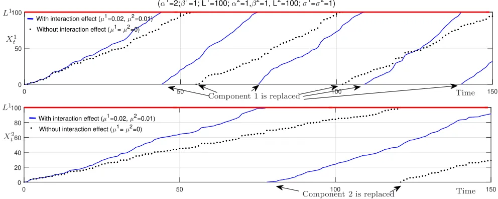
degradation rate of component i. Figure 1 illustrates the deterioration evolution of the two

dependent components. Note that when the deterioration of a component reaches its failure threshold, the component fails. We suppose that the failed component can be immediately

0 50 100 150 0

50 100

0 50 100 150

0 20 40 60 80 100

(α1=2;β1=1; L1=100; α2=1,β2=1, L2=100; σ1=σ2=1)

Without interaction effect (µ1= µ2=0) With interaction effect (µ1=0.02, µ2=0.01)

With interaction effect (µ1=0.02, µ2=0.01) Without interaction effect (µ1= µ2=0)

PSfrag replacements

Time Time

L1

L1

L2

X1 t

Xt2

Component 1 is replaced

Component 2 is replaced

Figure 1: Illustration of the deterioration evolution of two dependent components

It should be noted that the case 3 has been studied in [3] for prognostics of system lifetime,

in which a random intrinsic effect is considered and described by a Brownian motion process.

In the present paper, the use of the model (case 3) will be demonstrated and investigated

using a case study of a gearbox system consisting of two gears which is partially presented in

[1], see Section 4.

2.2

Economic dependence modelling

All necessary maintenance resources (such as spare parts, maintenance tools, repairmen) that are

required to execute maintenance actions are assumed always available at a planned inspection

time. It is also assumed that maintenance actions (replacements and inspections) are carried

out at discrete times. Replacements may be corrective (that is on failure of the system) or

preventive (prior to system failure) and that in the standard manner the costs differ in the two

cases.

2.2.1 Individual maintenance costs

If a preventive replacement is individually carried out, a preventive cost is then incurred. In

a general way, the preventive cost of component i, denoted Ci

p, can be divided into two parts:

Ci

p =cip+cd·di where cd·di is the downtime cost due to production loss during replacement

that takes di time units, and cip includes all other costs (spares, labour, set-up).

In the same manner, the cost of corrective replacement of component iis Ci

(ci c ≥cip).

Note, by preventive replacement of a component, we mean the replacement of a component

when it is unfailed, and by corrective replacement of a component, we mean the replacement of

a component when it is failed. Full details of the maintenance policy follow in section 3.

2.2.2 Economic dependence and cost saving

When two components are simultaneously replaced, total maintenance cost can be reduced

[21, 10, 32]. In our model, this cost saving arises from the sharing of the replacement set-up

cost and the reduction of replacement duration. In this way, we define the cost-saving of joint

replacement as

CS−,−=a·(c1−+c2−) +b·(d1+d2)·cd, (3)

where:

• ci

− (i= 1,2) could be either cip or cic, i.e. preventive or corrective; • a (0 ≤a < min(c1

−, c2−)/(c1−+c2−)) is the cost-saving factor for joint replacement of two

components. As is shown in [32], that the cost saving is typically equal to 5% of the total

replacement cost of the components (a= 0.05);

• b (0≤b≤min(d1, d2)/(d1+d2)) is the duration-saving factor for joint replacement.

In this way, a, b express the economic dependence degree between the two components. When

a = 0 and b = 0, the two components are economically independent. The larger are a and b

, the stronger is the economic dependence between the two components. Note, the effect of

economic dependence on the availability of a system is studied in [9].

It is important to note that, in our paper, the economic dependence is positive (CS−,−≥0).

However, in parallel or complex structure systems where a failure of a component or a group of

group of components may not lead to a failure of the system, the economic dependence may be

positive or negative, see [19, 30].

In our paper, the elements of the economic dependence are integrated into an opportunistic

maintenance model that is described next.

3

Maintenance policy

We assume that the degradation level of each component is measured at an inspection that

a component is assumed to be instantaneously revealed by a self-announcing mechanism, but

that replacement can commence only at the next inspection. In this way, the usual practical

requirement to prepare for a replacement is modelled while the system downtime due to failure

is known.

3.1

Description of the proposed maintenance policy

We assume that the two components of the system are inspected at regular time intervals with

inter-inspection interval ∆T. Note that ∆T is a decision variable which is to be optimized. More

precisely, for each component i(i= 1,2), the degradation level at inspection timesTk=k·∆T

(k= 1,2, ...) isXi Tk =x

i

Tk. The maintenance policy is as follows. For i= 1,2:

• if component i fails between (Tk−1, Tk) (when its degradation level reaches the failure

thresholdLi), then it is replaced at time Tk;

• if at time Tk, component i is still functioning, it is inspected. Based on the inspection

results and the preventive maintenance rules, a decision about whether or not component

i should be replaced at time Tk will be taken. We specify rules for individual preventive

replacement and for opportunistic preventive replacement.

Individual preventive replacement If the degradation level of component i (i= 1,2)

at timeTk is greater or equal to a fixed thresholdmip (xiTk ≥m

i

p), componentiis immediately

replaced. mi

p, called the preventive threshold of componenti, and is a decision variable to be

optimized.

Opportunistic replacement The main idea of the proposed opportunistic replacement

model is to capitalize on both the economic dependence and the stochastic dependence between

the two components. The economic dependence is manifest in the shared set-up and the

cost-saving therein. The stochastic dependence, through the term ∆Xij in equation (2), may also

incentivise (depending on the strength of the dependence) joint replacement. To this end, for

each component i, an opportunistic threshold, denoted mio (0 < mio ≤ mip), is introduced.

The opportunistic maintenance decision rule is the following. If component j (j = 1,2 and

j 6= i) is correctively replaced or selected to be preventively replaced at time Tk, componenti

is preventively replaced together with component j if the degradation level of component i is

such that xi Tk ≥m

i

0. The latter implies that the system is renewed at time Tk. mio (i= 1,2) is

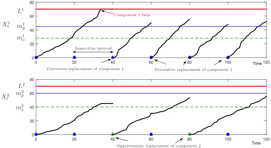
An illustration of the proposed opportunistic maintenance policy is shown in Figure 2.

0 20 40 60 80 100 120

0 20 40 60 80

0 20 40 60 80 100 120

0 20 40 60 80 Time Time PSfrag replacements

Corrective replacement of component 1 Preventive replacement of component 1 Component 1 fails

Inspection interval

Opportunistic replacement of component 2

L1 L2 m1 p m2 p m1 o m2 o X1 t X2 t

Degradation evolution of two components with maintenance actions

Figure 2: Illustration of components’ degradation evolution and the proposed maintenance policy

This general policy we label policy V. To study the impacts of opportunistic replacement,

two special cases of this policy are herein considered as follows

• When m1

p =m1o and m2p =m2o, there is no opportunistic replacement, the policy becomes

a classical condition-based maintenance policy [19] with discrete inspections, which we call

policy V1;

• When m1

o =m2o = 0, two components are jointly replaced together, the proposed policy

becomes a joint replacement policy, which we call policy V2.

To investigate the effects of economic and stochastic dependence, we compare the cost-rates

of these three policies V, V1 and V2 in Section 4.4.

3.2

Optimization of the proposed maintenance policy

As described, ( ∆T, m1

p, m1o, m2p, m2o) are the decision variables of the general opportunistic

replacement policy that we study. Their optimal values must be determined, given some suitable

criterion. For this purpose, a cost model is developed in this section. In particular, we use the

long-run expected cost per unit of time (or cost-rate) including replacement and inspection

The cost-rate is defined generally as:

C∞(∆T, m1_p, m1_o, m2_p, m2_o) = lim

t→∞

Ct_{(∆T, m}1

p, m2o, m2p, m2o)

t , (4)

whereCt_{(∆T, m}1

p, m2o, m2p, m2o) is the cumulative total maintenance (replacement and inspection)

cost in period (0 t]. According to the renewal theory [25], Eq. (4) can be rewritten as follows:

C∞(∆T, m1_p, m2_o, m2_p, m2_o) = E[C

Tre_{(∆T, m}1

p, m2o, m2p, m2o)] E[Tre]

, (5)

where E[.] is mathematical expectation and Tre is the length of the first renewal cycle of the

system, i.e. all components of the system are replaced at time Tre. Without losses of generality,

we assume that that Tre= ∆T·m (m is a positive integer), and so we get:

CTre_{(∆T, m}1

p, m2o, m2p, m2o) =

Pm

k=1(Cinsk +Cmaink ) +Tdown·cd

m·∆T ,

with:

• Ck

ins=u·cI withu (u= 0,1,2) being the number of components inspected atTk, noting

that failed components are not inspected;

• Ck

main=Cp1+Cp2−CSp,pif the two components are jointly, preventively replaced;Cmaink =

Ci

p if only component iis preventively replaced; Cmaink =Cpi+C j

c −CSp,c if componenti

is preventively replaced and component j (j 6=i) is correctively replaced; Ck

main =Cci if

only component i is correctively replaced and Ck

main = 0 if no replacement is performed

at Tk.

Obtaining a closed-form expression for the cost-rate in Equation (5) is very difficult or even

impossible. In [13], an efficient method based on semi-regenerative theory and Markov deci-sion processes is introduced to obtain a closed-form expresdeci-sion for the cost-rate of a single-unit

system with time-homogeneous degradation behavior. In [5], a similar technique is developed to calculate the cost-rate of a two-component system with time-homogeneous and independent degradation behavior. However, this analytical method cannot be applied when there is

degra-dation interaction between components. This is because, in presence of degradegra-dation interaction between components, the componentsˆa degradation process are dependent and non-longer

time-homogeneous. As a consequence, semi-regenerative theory and Markov decision processes

can-not be applied. Therefore, in our paper, the cost-rate is evaluated, given ∆T, m1p, m1o, m2p, m2o,

using Monte Carlo simulation. By varying the values of the decision variables and performing

an exhaustive, the minimum cost-rate can be identified.

C∞(∆T∗, m1p∗, m1o∗, m2p∗, m2o∗) = min{C∞(.)0<∆T,0 < m1

p ≤ L1,0 < m1o ≤ m1p,0 < m2p ≤L2,0 < m2o ≤m2p}.

4

Case study

Gearbox systems play an essential role in industrial machinery. They are widely used for torque

and speed conversion. Unforeseen gearbox failures cause downtime and production inefficiency,

leading to economic losses, and in some cases may have serious implications for safety. With

multiple interacting components, we would expect the degradation trajectories of each of the

components of a new gearbox, whereby all components are new, to be different to those of a

partially new gearbox, whereby some components are new. This stochastic dependence, and the

economic dependence arising from shared set-up costs, mean that an opportunistic maintenance

policy is appropriate. Therefore, in what follows, we show how the opportunistic replacement

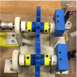
policy can be i) optimized and ii) used in practice. In particular, we study an accelerated-life

testing platform for a gearbox shown in Figure 3. This platform provides experimental data for

modelling the interacting degradation trajectories of two components in this system.

Figure 3: Gearbox system consisting of two interacting gears

4.1

Gearbox experimental scenario

The platform is driven by a DC motor running at 1200 RPM, and the load is provided via a

dynamometer system. The vibration signals of the gearbox were collected using accelerometers

and a data acquisition card which then transmitted the data to a PC workstation where they

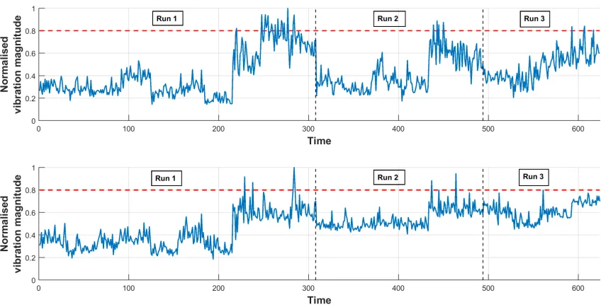
Data were collected in an experiment with three runs as follows:

Run 1: _{The first run of the gearbox was conducted until high system vibration was noticed.}

Destructive pitting occurred on the teeth surface of gear 1. It was therefore replaced with

a new gear, while gear 2 showed signs of initial pitting and was not replaced.

Run 2: _{The second run of the gearbox was then conducted until there was high system}

vibra-tion. The development of high vibration occurred over a shorter period of time.

Destruc-tive pitting occurred in gear 1, so it was replaced with a new gear. The condition of gear

2 showed more significant pitting in the second run but it was not replaced.

Run 3: _{The third and last run was then conducted until there was high system vibration. This}

occurred over an even shorter period of time than in the first two runs. The gearbox was

then stopped.

The degradation trajectories are shown in Figure 4.

Figure 4: Evolution of degradation of the gears in all three runs, represented by the mesh frequency magnitude

Some data processing of the vibration signals was required to arrive at the data in Figure 4.

We refer to gear 1 and 2 as component 1 (C1), and component 2 (C2) respectively. After

acquiring the vibration signal, we applied a short time Fourier transform on the time waveform

data and obtained spectrograms of the signals for C1 and C2. Then, using a dynamic frequency

an array of magnitudes for which we compute the root mean square (RMS). The RMS values

obtained over the full spectrogram summarise the time series data and are normalized and shown

in Figure 4. The RMS values inform us of the vibration energy in the machine that originates

from the gears. The higher the vibration energy the more the gears are deteriorated and the

more prone the gearbox is to damage. This proness of a gear to damage is the manifestation

in reality of the terms ∆Xii

t and ∆X

ij

t in the model (equation 2), the former because the gear

itself is worn, and the latter because the other gear is worn. We consider a component to be

severely worn out or to have failed once it reaches the threshold vibration magnitude ofLi _{= 0.8}

with i= 1,2.

It should be noted that the real data are scaled and all parameters are given in arbitrary

units, either arbitrary cost unit (acu) or arbitrary time unit (atu).

The inspection cost is 10 acu (cI = 10). When each gear is individually replaced, the

replacement cost and the maintenance duration are c1p =c1c = 500 acu, c2p =c2c = 600 acu and

d1 =d2 = 1 atu. When both gears are replaced together, 5% of the total replacement cost of the

components is saved (a= 0.05) and the total maintenance duration is reduced by 50% (b= 0.5).

In addition, when the system fails we have to pay 100 acu per downtime unit (cd = 100). The

downtime cost (due to system failure) is taken to be the (negative of the) average of the output

performance over the period of observation of the system, although in principle the downtime

cost could be specified in other ways.

4.2

State interaction modelling

Due to the physical characteristics of the gears, we know that the degradation level of

compo-nents C1 and C2 increases with time, and that this degradation level cannot decrease without

maintenance intervention. Therefore, both components are considered to have inherent

degra-dation that increases with time. We therefore assume that these degradegra-dation increments are

gamma-distributed (see Appendix A for more details). These increments are denoted by ∆X11

t

and ∆X22

t for C1 and C2 respectively. Thus, ∆Xt11∼Γ(α1, β1) and ∆Xt22∼Γ(α2, β2).

Next, we model the degradation interactions between the two components. It appears

(Fig-ure 4) that the state of C2 affects the rate of degradation of C1. This can be seen when we

observe the time to failure of C1 when coupled with a worn out C2 in runs 2 and 3, and that in

run 3, where C2 was more worn out, the time to failure of C1 was shorter than run 2. Thus the

degradation rate of C1 appears to be dependant on the degradation level of C2 and vice versa.

∆X21

increment in the degradation level of C2 due to C1.

We denote the degradation states for C1 and C2 at time t by X1

t and Xt2 respectively.

Further, since in our model ∆Xii

t >0 and ∆X ji

t >0, the state dependence model is as case 3

in section 2.1. Thus the evolution of degradation for C1 is described by:

Xt1 =Xt1−1+ ∆Xt1,

∆X_t1 = ∆X_t11+ ∆X_t21,

∆X_t1 = Γ(α1, β1) +µ1·(X_t2₋1)σ

1

.

and for C2 as:

X_t2 =X_t2₋₁+ ∆X_t2,

∆X_t2 = ∆X_t22+ ∆X_t12,

∆X_t2 = Γ(α2, β2) +µ2·(X_t1₋₁)σ2_.

Note that there exists four parameters that need to be estimated to describe the degradation

of each component. These parameters are denoted by Θ1 _{and Θ}2_{, where Θ}1 _{= (α}1_{, β}1_{, µ}1_{, σ}1₎

and Θ2_{= (α}2_{, β}2_{, µ}2_{, σ}2_{). In order to fit the degradation model to the data, we use the particle}

filter (PF) method [11]. PF allows for an online numerical estimation of the parameter values by means of a recursive Bayesian inference approach. The posterior distribution of the model

parameters can be then obtained using a number of particles and their corresponding weights. This method is very flexible and can be used for non-linear models where the noise is not

necessarily Gaussian. Such an approach has been successfully used in the field of prognostics for model parameter estimation [17, 22, 36]. The choice of PF is further motivated by the fact

that it is now considered a state of the art technique for performing diagnostics and prognostics [15].

To estimate Θ1 and Θ2 using PF, we start by specifying a number of particles np to use.

In our case we set np = 1000. Each particle is then associated with a value for each of the

four parameters, by sampling from a prior distribution. We use uniform distributions on the following intervals: Uα[0 0.1], Uβ[0 0.1], Uµ[0 0.1], Uσ[0 10]. The choice of these intervals is made

empirically, keeping in mind that a larger np means that different combinations of these

pa-rameters are more effectively explored. However, this would entail a larger computational cost.

the component ˜X_ti,n forn= 1 :np. Then, after observing the actual health condition yit we can

determine the importance weight of each particle by computing the likelihood of that

observa-tion given the predicted values of each particlep(yt|X˜ti,n). The weights are then normalized and

bootstrap-importance sampling (re-sampling with replacement np particles from the previous

set of particles according to their weights) is performed. This process is repeated using the new set of particles, as shown in Algorithm 1. After 308 iterations, we obtain the mean estimated

value of each parameter (Table 1). Note that since the degradation level is normalized between 0 and 1, the greater is the value of the parameter bi _{the smaller is the impact of the other}

component on componenti.

Algorithm 1: Particle Filter Algorithm input : np number of particles

Initialisation

t= 0

for i←1 to np do

Sample xi

0 ∼p(x0)

end

for t←1 to tend do

Importance Sampling

for i←1 to np do

Sample ˜xn

t ∼p(xt|xit−1) Set ˜xi

0:t= (xi0:t−1,x˜it)

end

for n←1 to np do

Evaluate importance weights ˜wn

t =p(yt|x˜nt)

end

Normalise importance weights ˜wn t

Particle Selection

for n←1 to np do

Considering ˜w_tn, re-sample with replacement np particles

end

Component αi _βi _µi _σi

C1 0.0233 0.0425 0.0995 7.6659

C2 0.0125 0.0914 0.0493 9.7375

Table 1: Estimated parameter values

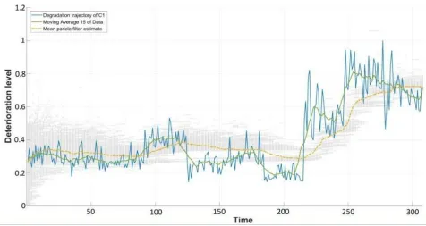
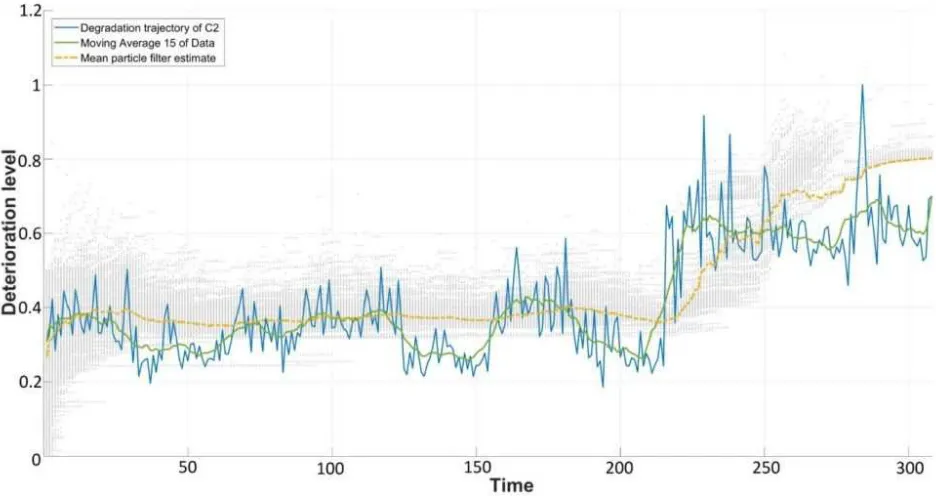
Figure 6: Fit of particle filter estimates to degradation data of component 2 in run 1

Figures 5 and 6 show the particle filter fit to the degradation data of run 1 for components 1 and 2 respectively. The grey dots represent the estimated degradation level at each time step

for each of thenpparticles. Therefore these grey dots representnp = 1000 different degradation

trajectories. The yellow dashed line represents the mean value of these trajectories at each time

step.

To further validate the parameter values of the degradation model considering the

interac-tions between the 2 components, we compute the R2 _{values for the fit of the average estimated}

degradation trajectory resulting from the particle filter to the real degradation trajectories. For

component 1 this is R2

1 = 0.792 and for component 2 it is R22 = 0.753. If we were to consider

a reduced model whereby no stochastic dependence is considered between the two components

and we are left with a gamma process describing the evolution of the degradation level for each

component, the average fit of such models results in anR2

1= 0.671 andR22 = 0.575. The further

advantage of considering the interactions between components is motivated in section 4.5.

Next, the fitted degradation model is integrated with the proposed maintenance model to

4.3

Optimum maintenance policy

To evaluate the cost-rate, a very large number of life cycles of the system were simulated

with above data. To find the optimal decision parameters (∆T, m1

p, m1o, m2p, m2o), the cost-rate

C∞(∆T, m1

p, m1o, m2p, m2o) is evaluated for different values of ∆T (∆T >0),m1p(0 < m1p ≤ L1),

m1

o (0 < m1o ≤ m1p), m2p (0 < mp2 ≤ L2) and m2o (0 < m2o ≤ m2p) using Equation (5).

The step size is 5 for the inter-inspection time, and 0.05 for each preventive or opportunistic threshold. With a precision of 0.010 specified for the rate, the convergence of the

cost-rate is reached from 10000 renewal cycles. The optimum values of the decision parameters are

∆T∗ _{= 60, m}1∗

p = 0.55, m1o∗ = 0.50, mp2∗ = 0.50 and m2o∗ = 0.40 with the minimum cost-rate

C∞(∆T∗, m1∗

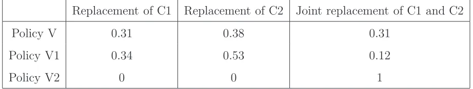
p , m1o∗, m2p∗, m2o∗) = 2.90 acu. Table 2 reports the proportion of maintenance

actions (replacement of C1 or C2; joint replacement of C1 and C2) at maintenance time for

each optimal maintenance policy. It should be noticed that two components are always replaced together in policy V2. The proportion of joint replacement in the proposed opportunistic

maintenance policy (policy V) is higher than in the non-opportunistic policy (policy V1). This is because the opportunistic thresholds tend towards a joint replacement of C1 and C2.

Replacement of C1 Replacement of C2 Joint replacement of C1 and C2

Policy V 0.31 0.38 0.31

Policy V1 0.34 0.53 0.12

Policy V2 0 0 1

0 20 40 60 80 100 120 140 160 180 200 2.5

3 3.5 4 4.5 5 5.5 6 6.5 7 7.5

Policy V Policy V1 Policy V2

PSfrag replacements

C

o

st

-r

a

te

∆T

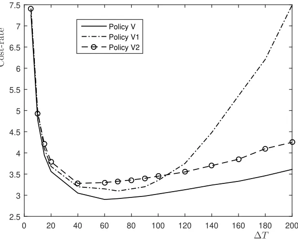
Figure 7: Cost-rate as a function of inter-inspection interval ∆T

Figure 7 shows the relationships between the minimum cost-rate and the inter-inspection

interval ∆T for the proposed opportunistic policy (policy V), non-opportunistic policy (policy

V1) and the joint replacement policy (policy V2). Each point represents an optimal policy with

a given value of ∆T.

This indicates that the proposed opportunistic maintenance policy (policy V) always provides

the lowest cost-rate. We observe that when ∆T <∆T∗ _{the maintenance cost increases rapidly}

and the difference between the three policies reduces with decreasing ∆T. However, when

∆T > ∆T∗_{, the cost-rate of the non-opportunistic policy (policy V1) increases rapidly with}

increasing ∆T, while the cost-rate of policies V and V2 increase slowly with increasing ∆T. This

indicates that the opportunistic replacement and the joint replacement can better compensate

for a sub-optimally large ∆T.

4.4

Impact of economic dependence on the cost

We now analyze the impact of economic dependence on the opportunistic replacement

mainte-nance policy. This is carried out by analyzing the sensitivity of the minimum cost-rate for three

policies V, V1 and V2 to the economic dependence degree (a, b) between the two components.

cost-rate of the proposed opportunistic policy V compared to policy Vi, denoted ∆Ci (i= 1,2), is

used. It is defined as follows:

∆Ci =

C_{V i}∞−C∞(∆T∗, m1∗

p , m1o∗, m2p∗, m2o∗)

C∞ V i

·100%

where C∞

V i is the minimum cost-rate of policy Vi with i = 1,2. According to the definition,

∆Ci>0 means that policy V is more effective than policy Viand less effective in the opposite

case.

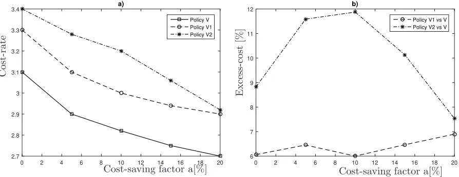
4.4.1 Sensitivity analysis to a

We vary a from 0 to 20% while the others parameters remain unchanged. For each value of

a the minimum cost-rate of each policy is determined and the excess-cost is then evaluated.

Summary results are shown in Figure 8.

0 2 4 6 8 10 12 14 16 18 20

2.7 2.8 2.9 3 3.1 3.2 3.3 3.4 a) Policy V Policy V1 Policy V2

0 2 4 6 8 10 12 14 16 18 20

6 7 8 9 10 11 12 b)

Policy V1 vs V Policy V2 vs V

PSfrag replacements C o st -r a te E x ce ss -c o st [% ]

Cost-saving factor a[%] Cost-saving factor a[%]

Figure 8: Cost-rate (a) and excess-cost (b) as a function of a

Figure 8(a) shows that the cost-rate decreases with the cost-saving factor a. This can be

explained by the fact that the maintenance costs reduce as aincreases. It is not surprising that

the proposed opportunistic policy V always provides a lowest cost-rate. This is because policies

V1 and V2 are two special cases of policy V.

Figure 8(b) shows that when a < 10% the excess-cost related to policy V2 increases with

an increasing of a. This means that the cost-rate of policy V2 decreases more slowly than

that of policy V as a increases. However, when a >10%, the cost-rate of policy V2 decreases

more rapidly than the cost-rate of policy V. While the cost-rate of policy V1 decreases more

slowly than that of policy V1 with increasinga. This can be explained by the fact that the two

To study more the impact of economic dependence degree on the maintenance cost, we

consider sensitivity with respect to the duration-saving factor b.

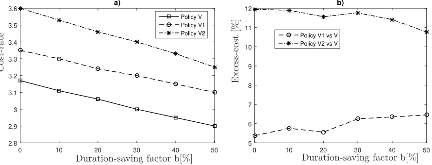
4.4.2 Sensitivity analysis to b

Here we varybfrom 0 to 50% while the others parameters remain unchanged. For each value of

b the minimum cost-rate of each maintenance policy is determined and the excess-cost is then

evaluated. The results obtained are shown in Figure 9.

0 10 20 30 40 50

2.8 2.9 3 3.1 3.2 3.3 3.4 3.5 3.6 a) Policy V Policy V1 Policy V2

0 10 20 30 40 50

5 6 7 8 9 10 11 12 b)

Policy V1 vs V Policy V2 vs V

PSfrag replacements C o st -r a te E x ce ss -c o st [% ]

Duration-saving factor b[%] Duration-saving factor b[%]

Figure 9: Cost-rate (a) and excess-cost (b) as a function of b

It is not surprising again that an increasing ofb(or equivalently a reduction on maintenance

duration when two components are replaced together) leads to a decreased cost-rate. However,

the effect for both the opportunistic policy (V) and non-opportunistic policy (V1) are broadly

the same, in a similar manner to that for varying a. This suggests that for both policies

there is a tendency that replacements of components are simultaneous. This is natural for

the opportunistic policy because this is its purpose. However we might have expected the

non-opportunistic policy to show less dependence on a and b. Our explanation for this is as

follows. When there is no opportunistic replacement, the threshold for preventive replacement

compensates (for component C1 in this case). It is lower (than with the opportunistic policy)

so that more often than not, the replacement of components is simultaneous (and set up cost

is saved). If it were not the case that replacements are simultaneous then the cost-rate for

policy V1 would not depend on a and b in the way it does. This effect only occurs because

of the positive stochastic dependence. If there was no positive stochastic dependence then

the simultaneous replacement of the components when one reaches a preventive replacement

Thus, when there is no stochastic dependence between components, opportunistic policies

become more effective as the extent of economic dependence increases. This is well known and

obvious. However, it would appear that when there is also positive stochastic dependence this

phenomenon is much less apparent. This is because a non-opportunistic policy will then

com-pensate for the absence of opportunities for replacement by lowering the threshold for preventive

replacement of the components. The positive stochastic dependence ensures that replacements

usually remain simultaneous because components will tend to cross their replacement

thresh-olds together. That said, this “deteriorating together” phenomenon will tend be more apparent

when the lifetimes of the components are broadly similar as is the case for the gearbox system.

4.4.3 Optimum policies when a= 0 and b= 0

We suppose now that two components are economically independent, i.e. a= 0 andb= 0. The

optimum maintenance policies are given in Table 3 where Pjoint indicates the probability that

two components are jointly replaced at each maintenance.

Optimum decision variables Pjoint Minimum cost-rate

Policy V ∆T∗_{= 60, m}1_∗

p = 0.6, m

1_∗

o = 0.55, m

2_∗

p = 0.5, m

2_∗

o = 0.45 0.18 3.22

Policy V1 ∆T∗_{= 60, m}1_∗

p = 0.6, m

2_∗

p = 0.5 0.12 3.26

Policy V2 ∆T∗_{= 50, m}1_∗

p = 0.55, m

2_∗

p = 0.65 1 3.69

Table 3: Optimum maintenance policies when a =b = 0

The obtained results show that when two components are economically independent, the

proposed opportunistic policy V is still slightly better than the non-opportunistic policy V1.

This is due to the opportunistic thresholds, which allow policy V to become more flexible

and better able to accommodate the stochastic dependence between components than the

non-opportunistic policy V1. However, the joint replacement (policy V2) has a higher cost-rate

which means that the joint replacement is not effective for this case.

4.5

Impacts of state dependence on the cost

To study the impact of state dependence between components on the optimum maintenance

policy, we assume now that the degradation process of each component evolves independently.

In this way, we reduce the degradation model to two independent gamma process for which the

shape and scale parameters can be estimated using maximum likelihood estimation (or using

Component αi _βi

C1 0.1165 0.0100

C2 0.0919 0.0090

Table 4: Estimated parameter values without considering stochastic dependence

The proposed maintenance policy is then applied. We obtained the optimal decision

vari-ables ∆T∗ = 120, m1∗

p = 0.60, m1o∗ = 0.45, mp2∗ = 0.55 and m2o∗ = 0.40. When compared

with the results obtained in Section 4.3, these optimal values are significantly different. In

addition, if we apply these optimal decision variables for the case considering the state

depen-dence between components, the cost-rate is then C∞_(∆T∗_{, m}1∗

p , m1o∗, m2p∗, m2o∗) = 3.75 acu.

This is significantly higher than the one obtained when the state dependence is considered in

degradation modeling ((3.75-2.90)/2.90)x100=29.3% higher). This implies that not considering

the state dependence between two components can lead to a sub-optimal maintenance policy.

Of course, the difference is itself dependent on the economic “dependence degree” between the

components.

5

Conclusions

In this work, a condition-based maintenance policy for a two-dependent component system is

studied. Two kinds of dependency are investigated and integrated in the maintenance modeling:

state dependence whereby the degradation rate of each component depends not only on its state

but on the state of the other component; and economic dependence whereby set-up cost and

duration are shared when components are replaced simultaneously. To select the components

to be preventively maintained at each inspection epoch, adaptive preventive replacement and

opportunistic replacement rules are proposed. A cost model taking into account the economic

dependence between components is developed to find the optimal values of the decision

vari-ables. The policies are studied in the context of a gearbox system consisting of gears. The

results indicate that (i) accounting for the state dependence between components is important,

and to ignore it has a significant impact ( 29.3%) on the cost; (ii) introducing an opportunistic

threshold for replacement makes the maintenance policy more flexible and less sensitive to a

sub-optimally large inspection interval; and (iii) when there exists positive stochastic

depen-dence between components so that components tend to deteriorate together, introducing an

is positive stochastic dependence between components than when there is not. This is because

replacements will tend to be synchronized and this tendency to synchronise arises precisely

because of degradation dependence. Thus we might claim a general insight that opportunistic maintenance is less opportune when components tend to deteriorate together than when they

do not. It will be very interesting to investigate this claim in a more general context, and this will be the subject of future work.

Finally, the proposed opportunistic maintenance policy might be extended to a larger system, but at the cost of exploring a much larger decision space and a significantly greater computation

time. The development of an analytical or efficient heuristic approach for the evaluation of the cost-rate then becomes important. It would also be interesting to apply the proposed

maintenance policy in a large-scale industrial case study. Another perspective should be the investigation on real time CBM vs inspection in presence of degradation interaction between

components.

Appendix

Appendix A. Gamma distribution

A random variable X which is gamma-distributed with shape αi _{and rateβ}i _{is denoted}

X∼Γ(αi, βi).

The corresponding probability density function (PDF) is

f_αi_,βi(x) =

1 Γ(αi₎ ·(β

i₎αi

·xαi−1·e−βi·x· I_{x≥0},

where:

• Γ(αi) =

+∞

Z

0

uαi−1·e−udu denotes a complete gamma function;

• I{x≥0} is an indicator function. I{x≥0}= 1 if x≥0, I{x≥0} = 0 and otherwise.

References

[1] R. Assaf, P. Do, P. Scarf, and S. Nefti-Meziani. Wear rate-state interaction modelling for

a multi-component system: Models and an experimental platform. IFAC-PapersOnLine,

[2] F. Barbera, H. Schneider, and E. Watson. A condition based maintenance model for a

two-unit series system. European Journal of Operational Research, 116:281–290, 1999.

[3] L. Bian and N. Gebraeel. Stochastic framework for partially degradation systems with

continuous component degradation-rate-interactions. Naval Research Logistics, 61:286–303,

2014.

[4] L. Bian and N. Gebraeel. Stochastic modeling and real-time prognostics for

multi-component systems with degradation rate interactions.IIE Transactions, 46:470–482, 2014.

[5] B. Castenier, A. Grall, and C. Berenguer. A condition-based maintenance policy with

non-periodic inspections for a two-unit series system. Reliability Engineering and System

Safety, 87:109–120, 2005.

[6] R. Dekker, L. Wildeman, and F. Van Der Duyn Schouten. A review of multi-component

maintenance models with economic dependence. Mathematical Methods of Operations

Re-search, 45(3):441–435, 1997.

[7] P. Do, P. Scarf, and B. Iung. Condition-based maintenance for a two-component system

with dependencies. IFAC-PapersOnLine, 48(21):946–951, 2015.

[8] P. Do, A. Voisin, E. Levrat, and B. Iung. A proactive condition-based maintenance strategy

with both perfect and imperfect maintenance actions. Reliability Engineering and System

Safety, 133:22–32, 2015.

[9] P. Do, H.-C. Vu, A. Barros, and C. Berenguer. Maintenance grouping for multi-component

systems with availability constraints and limited maintenance teams. Reliability

Engineer-ing and System Safety, 142:56–67, 2015.

[10] P. Do Van, A. Barros, C. Berenguer, K. Bouvard, and F. Brissaud. Dynamic grouping

maintenance strategy with time limited opportunities. Reliability Engineering and System

Safety, 120:51–59, 2013.

[11] A. Doucet and A. M. Johansen. A tutorial on particle filtering and smoothing: Fifteen

years later. Handbook of nonlinear filtering, 12(656-704):3, 2009.

[12] H. R. Golmakani and H. Moakedi. Periodic inspection optimization model for a

two-component repairable system with failure interaction. Computers and Industrial

Engineer-ing, 63(3):540–545, 2012.

[13] A. Grall, L. Dieulle, C. B´erenguer, and M. Roussignol. Continuous-time

predective-maintenance scheduling for a deteriorating system. IEEE Transactions On Reliability,

[14] B. Iung, P. Do, E. Levrat, and A. Voisin. Opportunistic maintenance based on

multi-dependent components of manufacturing systems. CIRP Annals Manufacturing

Technol-ogy, 65(1):401–404, 2016.

[15] M. Jouin, R. Gouriveau, D. Hissel, M.-C. P´era, and N. Zerhouni. Particle filter-based

prog-nostics: Review, discussion and perspectives. Mechanical Systems and Signal Processing,

72:2–31, 2016.

[16] M. C. O. Keizer, S. D. P. Flapper, and R. H. Teunter. Condition-based maintenance

policies for systems with multiple dependent components: A review. European Journal of

Operational Research, 261(1):405–420, 2017.

[17] P. Li, R. Goodall, and V. Kadirkamanathan. Parameter estimation of railway vehicle

dynamic model using rao-blackwellised particle filter. In European Control Conference

(ECC), 2003, pages 2384–2389. IEEE, 2003.

[18] L. Liu, M. Yu, Y. Maa, and Y. Tu. Economic and economic-statistical designs of an

x control chart for two-unit series systems with condition-based maintenance. European

Journal of Operational Research, 226:491–499, 2013.

[19] K.-A. Nguyen, P. Do, and A. Grall. Condition-based maintenance for multi-component

systems using importance measure and predictive information. International Journal of

Systems Science: Operations & Logistics, 1(4):228–45, 2014.

[20] K.-A. Nguyen, P. Do, and A. Grall. Multi-level predictive maintenance for multi-component

systems. Reliability Engineering and System Safety, 44:83–94, 2015.

[21] R. Nicolai and R. Dekker. Optimal maintenance of multi-component systems: a review.

Complex System Maintenance Handbook, London: Springer, pages 263–286, 2008.

[22] M. E. Orchard and G. J. Vachtsevanos. A particle-filtering approach for on-line fault

diagnosis and failure prognosis. Transactions of the Institute of Measurement and Control,

31(3-4):221–246, 2009.

[23] N. Rasmekomen and A. Parlikad. Condition-based maintenance of multi-component

sys-tems with degradation state-rate interactions. Reliability Engineering and System Safety,

148:1–10, 2016.

[24] N. Rasmekomen and A. K. Parlikad. Optimising maintenance of multi-component systems

with degradation interactions. In Proceedings of the 19th IFAC World Congress, 2014,

[25] S. Ross. Stochastic Processes. Wiley Series in Probability and Statistics. John Wiley and

Sons, Inc., 1996.

[26] P. Scarf and M. Deara. Block replacement policies for a two-component system with failure

dependence. Naval Research Logistics, 50:70–87, 2003.

[27] X. Si, W. Wang, , C. Hu, D.-H. Zhou, and M.-G. Pecht. Remaining useful life estimation

based on a nonlinear diffusion degradation processn. IEEE Transactions on reliability,

6:50–67, 2012.

[28] F. van der Duyn Schouten and S. Vanneste. Analysis and computation of( n, n)-strategies

for maintenance of a two component system. European Journal of Operational Research,

48:260–274, 1990.

[29] J. Van Noortwijk. A survey of the application of Gamma processes in maintenance.

Reli-ability Engineering and System Safety, 94:2–21, 2009.

[30] H.-C. Vu, P. Do, A. Barros, and C. Berenguer. Maintenance grouping strategy for

multi-component systems with dynamic contexts. Reliability Engineering and System Safety,

132:233–249, 2014.

[31] H. Wang. A survey of maintenance policies of deteriorating systems. European journal of

operational research, 139(3):469–489, 2002.

[32] R. Wildeman, R. Dekker, and A. Smit. A dynamic policy for grouping maintenance

activ-ities. European Journal of Operational Research, 99:530–551, 1997.

[33] S. Wu and P. Scarf. Two new stochastic models of the failure process of a series system.

European Journal of Operational Research, 257(3):763–772, 2017.

[34] S. Wu and J. M. Zuo. Linear and nonlinear preventive maintenance models. IEEE

Trans-actions On Reliability, 59(1):242–249, 2010.

[35] N. Zhang, M. Fouladirad, and A. Barros. Warranty analysis of a two-component system

with type i stochastic dependence. Proceedings of the Institution of Mechanical Engineers,

Part O: Journal of Risk and Reliability, 2017.

[36] E. Zio and G. Peloni. Particle filtering prognostic estimation of the remaining useful life