Optimizing the Data Collection in Wireless Sensor Network

© 2016, IRJET | Impact Factor value: 4.45 | ISO 9001:2008 Certified Journal

| Page 701

Optimizing the Data Collection in Wireless Sensor Network

R.Latha

_{,Valarmathi.M}

1

_{Assistant Professor,}

_{PG Scholar}

_{Computer Application}

1,2

_{Vel Tech High Tech DR.Rangarajan DR.Sakunthala Engineering College}

---***---

Abstract -

Key Words: Wireless Sensor Networks, Breadth First

Search, Parallel data collection, Binary tree.

1. INTRODUCTION

Sensor node is a small device to sense, receive and forward packets to its neighbor node. A tree rooted at a sink node is called data gathering tree, if every internal collects the data from sensors that are its child nodes and send this packet to its parent node. Finally the whole data is send to the sink for further processing. The sensor nodes and the sink are deployed in a geographical area and a binary tree structure is constructed. This is many to one data collection, so data collection scheduling is very important. So that there is a possibility of maximizing the data collection at sink.

Consider n sensor nodes, these n nodes are randomly deployed in a geographical area of m*m. n sensor nodes and a sink as root forms a Tree. At regular intervals, sink node collects sensed data from these n sensor nodes. After collecting, analyze the data collection capacity of the sink. As the main aim of this project is to minimize the delay and maximize the capacity. To achieve this, follow BFS data collection following three models. The three models are Disk Graph Model, Generalized Quasi Disk Graph Model and Protocol Interference Model.

Following these three models, collect data and send data to the sink node following BFS [1] approach. Capacity analysis is done in the sink. The capacity analysis is the amount of data sink can collect for a snapshot. Implementing BFS, the data collected and the delay required collecting data is analyzed. Each sensor node measures independent field values at regular time intervals and sends these values to sink node. The union of all these sensing values from n sensors at a particular time is called snapshot. Delay of Data collection D is the time used by the sink to successfully receive a snapshot, i.e., the time needed between completely receiving one snapshot and next snapshot at the sink.

Distance between the sensor nodes will be different and the amount of data to send will differ, so the energy utilized to send the data will differ for different sensor nodes. So each sensor node calculates the energy on its own. Each sensor node calculates the distance and energy to transfer data. Now three models mentioned above are implemented and traverse the nodes parallel and collect data parallely from nodes. This is Parallel Data Collection in BFS (PDCBFS). In BFS, individual packets (its own and its child nodes) are sent separately, but in PDCBFS every node aggregates the packets (its own and its child node) into a single packet and send to parent node. The amount of data collected and the delay required collecting data is analyzed.

Now performance analysis of data collected and delay required to collect data for both BFS and PDCBFS is done which shows the result of best of two algorithms (BFS and PDCBFS).

2. RELEVANT WORK

This paper focuses on data collection in WSN using parallel data collection in BFS. This section gives an idea of related data collection algorithms.

© 2016, IRJET | Impact Factor value: 4.45 | ISO 9001:2008 Certified Journal

| Page 702

of data collection is θ(W). Note that even for individual sensors, the lowest achievable delay rate of this method is θ(W=n) which also meets the upper bound.

Siyuan Chen, Shaojie Tang, Minsu Huang, Yu Wang [1] studied the capacity of data collection in an arbitrary network. They derived the upper and constructive lower bounds of data collection capacity in arbitrary networks. The BFS data collection method and path scheduling algorithm [1] achieved an upper bound of θ (W). They also examined the design of data collection under a general graph model and discuss performance implications.

Mahajan and J. Malhotra [2] used BFS approach for path determination. Breadth-First Search (BFS) is a node search algorithm that begins at the root node and explores all the neighboring nodes. Then for each of those nearest nodes in graph, it explores their unexplored neighbor nodes, and so on, until it finds the goal. It has been proved by induction that the BFS tree is a shortest path tree starting from its root. Every vertex has a path to the root, with it's path length equal to its level (just follow the tree itself), and no path can skip a level so this really is a shortest path. In both [1] and [2], they proved that BFS data collection have achieved a maximum data collection.

Barton and Rong [4] investigated the capacity of data collection under general physical layer models for example, cooperative time reversal communication model where the data rate of an individual link is not fixed as a constant W but dependent on the transmitting powers and distances of all simultaneous transmissions.

P. Balamurugan, K. Duraiswamy [9] gave a random rank to the vertices of the nodes between 0 and 1. A link is formed between any two nodes if they are within their transmission range. If a sensor node has the highest rank among its neighbors, then it is considered an associate node, else it forms into the leaf node. Next, the associate nodes form a complete graph and later form a Rooted Directed Tree (RDT) after an implementation of Kruskal’s Minimum Spanning Tree algorithm and the Breadth First Search algorithm. The energy consumption model is followed.

Firstly, a virtual tree topology is constructed based on Grid-based WSNs [12]. Then two node-placement techniques, namely Distance-based and Density-based deployment schemes are followed to balance the power consumption of sensor nodes. Finally, a collision-free MAC scheduling protocol [12] is proposed to prevent the packet transmissions from collision. In addition, extension of the proposed protocols is made from a Grid-based WSN to a randomly deployed WSN, enabling the energy-balanced schemes as they are generally applied to randomly deployed WSNs.

3. NETWORK MODEL

In [12], a N * N Grid-based WSN is considered, which consists of a sink node and -1 sensor nodes. Fig.1 shows a 3 * 3 Grid-based topology composed of a sink node and = 8 sensor nodes.

Figure 1: Grid based topology

In Fig 1.the Sink is placed in the coordinate (1,1) top right position and the coordinate of each sensor node is increased by 1 when moves left in x-axis and increased by 1 when moves down in y-axis. Fig. 1 shows the constructed root-balanced tree which is rooted by sink.

3.1 Grid based WSN

For an example, Grid based topology is formed with a sink node and six sensor nodes. Then a tree structure of this Grid based topology is identified. In [12], the tree constructed guarantees that the numbers of nodes in left and right sub-trees of the sink node differ one at most had been proved. This Grid based WSN is identified as tree structure.

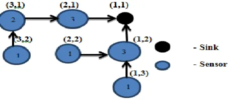
Figure 2: Sample Grid based WSN

Numbers in the sensor node denotes how many packets a node would have to send to the sink. This will be calculated by the sink. Based on the number of packets, power required by the sensor node differs. This will be discussed in section 4. The coordinates shown in fig. 2 are logical coordinates. In this paper, the logical coordinates of the Grid based WSN are not converted to physical coordinates. The physical coordinates of the nodes are initially given as input to geographically deploy the nodes.

3.2 Tree construction of WSN

© 2016, IRJET | Impact Factor value: 4.45 | ISO 9001:2008 Certified Journal

| Page 703

sensor nodes. Consider n nodes in the graph. For example assume that the sensor nodes and sink are deployed over a geographical area of 2000*2000 and there are 100 Sensor Nodes spread in the geographical area of 2000*2000. At regular intervals, sensor nodes generate b bits and want to send it to the sink. The union of data from sensor nodes at this regular interval is called snapshot. The data size of one snapshot is n*b.

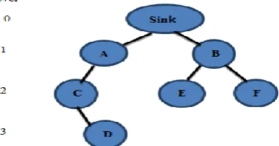
Figure 3: Tree structure of sensor nodes

In Fig. 3, A, B, C, D, E, F are the sensor nodes. Figure 3 shows the tree structure of six sensor nodes and one sink node formed from the Grid based WSN in Fig 2 and they are placed at the coordinates mentioned in the table 1.

Node A B C D E F Sink

X-coordinate

Y-Coordinate

50

90 120

80 20

30 70

10 80

20 180

40 100

190

Table 1: Coordinates of Sensor Nodes

This Coordinates are used to find distance between the sensor nodes. The distance is calculated based on the coordinates given in table 1.

Nodes Distance (meters)

C to A D to C E to B F to B A to Sink B to Sink

67.1 53.9 72.1 72.1 50 22.7

Table 2: Distance between the Sensor Nodes in fig. 3

Based on the distance calculated in table 2, the energy required by the sensor nodes is calculated. The energy calculation formula is given in table 3.

4. MODELS

4.1 Disk Graph Model

A sensor node sends or receives data from or to another sensor node if that sensor node is within a range. This is Disk Graph Model. Here fix a range r for all sensor nodes. A sensor node can transfer data to another sensor node

if

| - |<=r Cannot transfer data to if

| - |>r

and are the locations of the sensor nodes.

Algorithm for Disk Graph Model:

1. INPUT: Graph G (V, E), root as sink s and range r. 2. Dg=0

3. For each sensor node

4. Find the neighbor nodes of the sensor nodes 5. For each neighbor node

6. Find distance d between the sensor nodes 7. If d<=r then

8. Dg=1 9. End if 10. End For 11. End For

4.2 Protocol Interference Model

A sensor node can send to sensor node if no other sensor node is sending data simultaneously within the interference range. This is Protocol Interference Model. A sensor node can successfully transfer data to a sensor node if

| - | ≤ R

and for any other simultaneously transmitting node , | - | ≥ (1 + Δ)R

© 2016, IRJET | Impact Factor value: 4.45 | ISO 9001:2008 Certified Journal

| Page 704

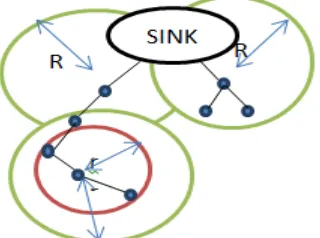
In the fig. 4, dots denote the sensor nodes. r is the range within which a sensor node can communicate with other sensor nodes. R is the interference range in which two sensor nodes in the same interference range R cannot send data to its neighbor node simultaneously to avoid collision. That is only one node in range R will be in active state.

4.3 Generalized Quasi Disk Graph Model

One extension of the DG model is to consider nodes in R3. Moreover, distances between nodes could be modeled using the Manhattan norm (L1 norm). In the Manhattan norm, the distance between two points u = ( , ) and v = ( , ) in the plane is given by d(u, v) = | − | + | − |, while in the Euclidean norm (L2 norm), the distance is

d(u, v) = + . Alternatively, the

maximum norm(L∞ norm) is also popular, where d(u, v) = max | − |, | − |. Distance can be calculated using any of the above mentioned norms.

5. ENERGY CALCULATION

The lifetime of a sensor node depends on its power (energy). Power required by the sensor nodes differs from sensor node to sensor node. It depends on its position that is how close the sensor node is from the sink.

This work uses the following energy consumption model for all the sensor-network related projects [9].

Table 3: Energy calculation

The transmitter amplifier energy cost is to achieve an acceptable Signal-to-noise ratio so that the signal received can be processed

Let data size be k = 512 bits

Energy lost at C = Energy lost to receive + Energy lost to transmit =230523.4 nJ

Energy lost at D = 374080.0 nJ Energy lost at E = 291758.6 nJ Energy lost at F = 291758.6 nJ

Energy lost at A = Energy lost to receive + Energy lost to transmit = 179200.0 nJ

Energy lost at B = Energy lost to receive + Energy lost to transmit = 77582.9 nJ

Total Energy Lost in the Network = 1444903.5 nJ = 0.00144J

Nodes Energy lost at nodes (nJ) C

D E F A B

230523.4 374080.0 291758.6 291758.6 179200.0 77582.9

Table 4: Energy required by the Sensor Nodes in Fig. 1

Using the X and Y coordinates, the distance between the sensor nodes is calculated and then the energy required by each sensor node is calculated, based on its activities. If a sensor node is a child node, then it consumes energy only to transfer the packets. If a sensor node is a parent node, then it requires energy to receive the packets from its child nodes, energy to integrate the packets and energy to transfer the packets to its parent. Based on these conditions each sensor node calculates the distance from its neighbor node and the energy it require.

6. DATA COLLECTION

6.1 BFS Data Collection

Breadth-first search (BFS) which is a Graph search algorithm in graph theory that begins at the root node and explores all the neighbor nodes. For each of those nearest nodes, it explores their unexplored neighbor nodes, and so on, until it finds the goal node. It has been proved by induction that the breadth first search tree is a shortest path tree starting from its root. Every vertex in tree has a path to the root, with path length equal to its level, and no path can skip a level so this really is a shortest path.

Operation Energy Dissipated

Transmitter Electronics( ETx-elec)

Receiver Electronics(

ERx-elec)

(ETx-elec = ERx-elec = Eelec) Transmitter Amplifier(ɛamp) To transmit a message of size k-bits, over distance d m To receive a k-bit message Cost for data fusion

50 nJ/ bit

100 pJ/ bit/

ETx(k, d) = Eelec * k + ɛamp * k *

© 2016, IRJET | Impact Factor value: 4.45 | ISO 9001:2008 Certified Journal

| Page 705

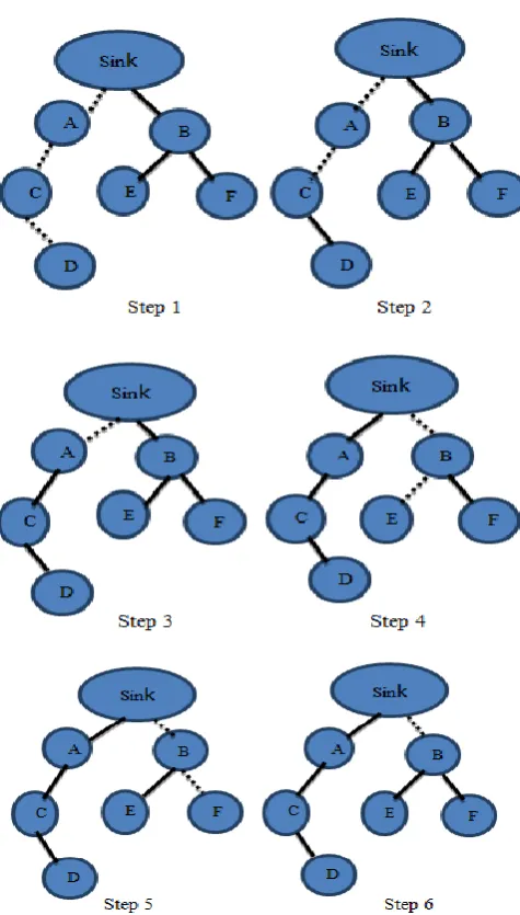
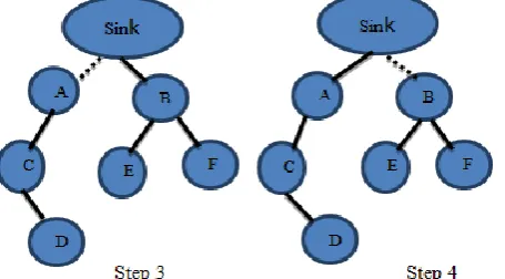
In the fig. 5, it shows the data collection based on BFS (Breadth first Search). Dotted line represents the exploring nodes; plain lines represent the link between the sensor nodes. The sink starts searching its first child and explores its neighbor nodes in step 1 and step 2. Node D sends data to node C and node C tags its data and node D’s data and send to node A. In step 3, node A tags its data to the received data and send to the sink. In step 4, it searches its next child node and explores its own child nodes E and F in step 4 and step 5. This data is buffered in node B and in step 6 this data is send to the sink. This completes a snapshot. The network link has a capacity to send or receive t bits/sec. The snapshot is divided into time slots.

Siyuan Chen, Shaojie Tang [1] studied that the BFS-based data collection method can achieve data collection capacity of θ(W) at the sink. They proved that data collection capacity is θ(W).

Figure 6: Time slots required for BFS data collection

The fig. 6 shows the time slots to complete a snapshot. Numbers on arrow denotes the time slots it requires to send the data to its parent node. The worst case is considered that is every node sends t bit/sec to its parent that is, it utilizes the complete data rate of a link. That is why nodes D, E, F require one time slot to send the data to its parent. Node C requires two time slots to send data to A because it has buffered t data from D and its own data t bits so it requires two time slots. Node A requires three time slots to send the data to the sink because it has buffered 2t data from node C, D and its own data t bits so it requires three time slots. This is the case for node B. Total time slots required to complete a snapshot is 1+2+3+1+1+3=11 time slots. A network with six nodes requires eleven time slots to complete a snapshot.

6.2 Parallel Data collection in BFS

© 2016, IRJET | Impact Factor value: 4.45 | ISO 9001:2008 Certified Journal

| Page 706

In step 1, the sink starts searching all its child nodes in parallel. It explores its child node, this child nodes explores its child nodes simultaneously. That is from the fig. 7 in step 1, node D sends the data to its parent node. Node C aggregates its own data with the node D’s data and node E sends data to node B. In step 2, node C and node F send data to its parent node. The data is buffered at their parent nodes. In step 3, node A sends data to the sink. In step 4, node B sends data to sink.

Data buffered and this data is aggregated and send this as a single packet. There is not much work on capacity of data aggregation in wireless sensor networks, except in recent papers [10] and [11]. Giridhar and Kumar [10] investigated a more general aggregation problem in random sensor network where a symmetric function of sensor measurements is used for data aggregation in WSN. It was shown that for random planar multi-hop network, the maximum rate for computing divisible functions (i.e., a

subset of symmetric functions) is θ ( W). Notice that they defined the maximum rate as the data rate per sensor. In addition, using a technique called block coding, they further showed that type-threshold functions can be

computed at a rate of θ ( W). Moscibroda [11] then further studied the aggregation capacity for arbitrarily deployed networks (he called this as worst-case capacity) under both protocol interference model and physical interference model. He showed that the worst-case

capacities of data aggregation are θ ( W) and Ω( ) respectively.

Figure 8: Time slots required for parallel data collection in BFS

By following parallel data collection in BFS, time slots less than the time slots required for normal BFS is achieved. Fig. 8 shows that node C and node E together require one time slot to send data to its parent node. Node A and node B each requires one time slots to send data to the sink because it aggregates the packets into a single packet during transmission. Total time slots require are 1+1+1+1+1=5 time slots to complete a snapshot. Previously BFS achieved eleven time slots to complete a snapshot. With six nodes in a network, it got six time slots difference. If the network grows, then there will be a drastic difference between the time slots utilized.

Here comes the conclusion that, parallel data collection in BFS gives the optimal data collection in WSN.

Barton and Rong [4] investigated the capacity of data collection under general physical layer models (e.g. cooperative time reversal communication model) where the data rate of an individual link is not fixed as a constant W but dependent on the transmitting powers and distances of all simultaneous transmissions. To calculate the transmitting power, the energy required for each and every node is calculated. Based on this study, the data rate of the links is not fixed as a constant W. Then the time slots required by all sensor nodes will become one time slot even though they are having many packets to send. Following this aggregation of packets into single packet, in above example it takes only five time slots to complete a snapshot.

Node T[N] Child T[C] Parent T[P]

Sink T[R] A B C

A,B C E,F

D

- Sink Sink A Table 5: Relationship between nodes

© 2016, IRJET | Impact Factor value: 4.45 | ISO 9001:2008 Certified Journal

| Page 707

Algorithm for Time slot calculation in Parallel Data collection in BFS

1. INPUT: Graph G (V,E), range r 2. Data = 0

3. At time = 0 For each T[R]->T[C] 4. time slot TS=0

5. For each T[N] 6. For each T[C] 7. TS++

8. Data = Data + data of T[C] 9. End For

10. End For 11. End For

7. DATA COLLECTION ANALYSIS AT SINK

(for parallel data collection)

Let total time slot required to collect a snapshot be T. T= α.τ + ( C – 1 ) is the at most time slot required. Here α denotes level of the tree, τ is the max of the time slot required by a node. Time slot required by a node t = b/W , b is the bits to transfer, W is the maximum transfer rate of a node, τ = max(t1,t2………tn). C is the number of child nodes a Sink have. Delay of data collection D = (α + (C-1)) τ. Delay of data collection is minimized by using parallel data collection in Network. After data collection for one snapshot, data collection capacity analysis is done at the sink node. Data collection Capacity C = n*b/D, here n is the number of Sensor Nodes, b is number of bits each Sensor Node can transfer, D is the delay between the snapshots.

So C = = . Here α, C are

constants. So the upper bound of θ (W) is obtained, by this derivation the upper bound is achieved. Thus the data collection in sink is maximized.

8. PERFORMANCE ANALYSIS

Nodes are placed randomly and uniformly in given geographical area. The energy required to transfer the data for each and every node is calculated. The distance between the nodes is calculated using any of the three norms (GQDG model) formula. After setting up this, data is collected using BFS and PDCBFS algorithm.

In BFS algorithm, parent nodes receives the packet individually and when a node sends data no other node in the network transmits the data which takes more time (delay) for sink to collect the data. But in PDCBFS algorithm, parent node combines packets to one packet and transmits to its parent and nodes transmit data parallely without collision. To avoid the collision Protocol Interference Model is implemented.

Data is collected using both these algorithms (BFS and PDCBFS). Analysis is done for a snapshot. Data collected for one snapshot and delay taken to collect a snapshot is calculated in sink. This calculation is done separately for both these algorithms. Graph is plotted for both data collected and delay taken. This analysis is done deploying the nodes uniformly and randomly. First two graphs for uniform placement of nodes and second two graphs for random placement of nodes in geographical area.

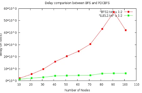
Figure 9: Graph to compare the delay for uniformly placed nodes

Fig. 9 shows the comparison of delay taken by BFS and PDCBFS for uniformly placed nodes. This graph shows that PDCBFS takes much less delay than BFS and there is only a moderate increase in the delay for PDCBFS. But in BFS, after 40 nodes very fast increase in the delay is found. This shows that delay taken for PDCBFS to collect data is much less than BFS algorithm.

Figure 10: Graph to compare data collected for uniformly placed nodes

© 2016, IRJET | Impact Factor value: 4.45 | ISO 9001:2008 Certified Journal

| Page 708

placed nodes

Fig. 11 shows the comparison of delay taken by BFS and PDCBFS for randomly placed nodes. This graph shows that PDCBFS takes much less delay than BFS and there is only a moderate increase in the delay for PDCBFS. But in BFS, after 70 nodes very fast increase in the delay is found. This shows that delay taken for PDCBFS to collect data is much less than BFS algorithm.

Figure 12: Graph to compare data collected for uniformly placed nodes

Fig. 12 shows the comparison of data collected by BFS and PDCBFS for randomly placed nodes. This graph shows that PDCBFS has collected more data than BFS. In BFS, after 40 nodes there is no increase in the amount of data collected but in PDCBFS, only after 80 nodes there is no increase in the amount of data collected. Graph 10 shows that the PDCBFS is much better than BFS in data collection. From these graphs, the conclusion is clear that parallel data collection in BFS algorithm collects more data than in less delay when compared to BFS algorithm. And it is already proved that PDCBFS collects data with an upper bound of θ (nW) which is exceeded the upper bound θ (W) of BFS algorithm.

9. CONCLUSION

In this paper, a tree structure of Wireless Sensor Networks is constructed. The distance between the sensor nodes and

energy needed by the sensor nodes to transfer and receive the data is calculated. The distance and energy to achieve the link data rate is calculated so that the data from different sensor nodes can be buffered and aggregated into a single packet and send through that link. First data is collected using BFS and data collected in a snapshot and the time slots required to collect a snapshot is calculated. In [1], an upper bound of θ (W) for data collection is achieved. In this paper, the data is collected parallely using BFS approach and send to the sink and the data collected in a snapshot and the time slots required for a snapshot is calculated. This is implemented deploying the nodes randomly and uniformly in a geographical area. This statistics of data collected and delay taken to collect a snapshot is analyzed using graph. From that graphs, it has been proved that parallel data collection in BFS collects more data in less delay than BFS algorithm. By this work, the upper bound is exceeded which has been achieved using BFS algorithm; this has been proved in previous section.

As this work is based on TDMA and energy calculation, if any node stops responding it can lead to total failure of the network. So a secondary parent to every node is deployed so that if any parent node stops working then the child node can transfer the data to its secondary parent. But the secondary parent does not simulate the parent. It does not sense the data but receive the data from the child node and transfer that data to its parent node. Then the network works smoothly all the time. This will be our future work.

REFERENCES

[1] Siyuan Chen, Shaojie Tang, Minsu Huang, Yu

Wang, “Capacity of Data Collection in Arbitrary Wireless Sensor Networks”, IEEE Computer Society, Jan 2012.

[2] Mahajan and J. Malhotra, "Energy Efficient Path

Determination in Wireless Sensor Network Using BFS Approach“, Wireless Sensor Network, Vol. 3 No. 11, 2011, pp. 351-356. doi: 10.4236/wsn.2011.311040.

[3] P. Gupta and P.R. Kumar, “The Capacity of

Wireless Networks”, IEEE Transactions on Information Theory, vol.46, no. 2, pp. 388–404, March 2000.

[4] R. Zheng and R.J. Barton, “Toward optimal data

aggregation in random wireless sensor networks,” in Proc. of IEEE Conference on Computer Communications (Infocom), 2007.

[5] X.-Y. Li, Y. Wang, and Y. Wang, “Complexity of Data

Collection, Aggregation, and Selection for Wireless Sensor Networks,” IEEE Trans. Computers, vol. 60, no. 3, pp. 386-399, Mar. 2011.

[6] “Fault-tolerant Scheduling for Data Collection in

© 2016, IRJET | Impact Factor value: 4.45 | ISO 9001:2008 Certified Journal

| Page 709

Anil Sarje, 2012 International Conference, pg No. 382-386.

[7] Enrique J. Duarte-Melo and Mingyan Liu,

“Data-gathering wireless sensor networks: Organization and capacity,” Computer

Networks, vol.43, pp. 519–537, 2003.

[8] Mingyan Liu David L. Neuhoff Daniel Marco,

Enrique J. Duarte-Melo, “On the many-to-one transport capacity of a dense wireless sensor network and the compressibility of its data,” in Proc. of International Workshop on Information Processing in Sensor Networks, 2003.

[9] P. Balamurugan, K. Duraiswamy, “Evaluation of

Energy and Delay Computing Algorithm for Data Gathering in Wireless Sensor Networks”,

European Journal of Scientific Research, ISSN 1450-216X Vol.66 No.1 (2011), pp. 85-95.

[10] A. Giridhar and P.R. Kumar, “Computing and

communicating functions over sensor networks,”

IEEE Journal on Selected Areas in Communications,

vol. 23, no. 4, pp. 755–764, 2005.

[11]Thomas Moscibroda, “The worst-case capacity of

wireless sensor networks,” in IPSN ’07: Proceedings of the 6th international conference on

Information processing in sensor networks, 2007.

[12] Chih-Yung Chang, Hsu-Ruey Chang,