A practical system to predict the absorption coefficient, dimension and reverberation time of room using GLCM, DVP and neural network

International Conference on Mechanical Engineering Research (ICMER2013), 1-3 July 2013 Bukit Gambang Resort City, Kuantan, Pahang, Malaysia Organized by Faculty of Mechanical Engineering, Universiti Malaysia Pahang Paper ID: P049

1

A PRACTICAL SYSTEM TO PREDICT THE ABSORPTION COEFFICIENT, DIMENSION AND REVERBERATION TIME OF ROOM USING GLCM, DVP

AND NEURAL NETWORK

M.N. Yahya1,2, T. Otsuru2, R. Tomiku2, T. Okuzono2

1

Faculty of Mechanical and Manufacturing Engineering, UTHM 86400, Parit Raja, Batu Pahat, Johor Malaysia

Phone : +607-453-7742 ; Fax : +607-453-6080 Email: [email protected]

2

Dept. Of Architecture and Mechatronic, Fac. of Engineering, Oita University, 700 Dannoharu, Oita 870-1192, Japan

Email: [email protected],jp, [email protected], [email protected]

ABSTRACT

In various prediction techniques of reverberation time such as Sabine and Eyring equation, ray-method, and numerical method require main parameters such absorption coefficient and dimensions. Normally, these parameters are obtained from references or/and measurements that necessitate special equipment and skills. On that matters, the authors have proposed a new practical technique to identify absorption coefficient and dimension of rooms. The technique comprises Subsystem_1 and Subsystem_2, each of which uses photographic images. Subsystem_1 uses a Gray Level Co-occurrence Matrix (GLCM) and integrate with Neural Network (NN) to identify the absorption coefficient of material. While, Subsystem_2 uses Dimension Vision Predictor (DVP) with the author’s “ruler method” to identify the dimensions. Examinations conducted in practical rooms revealed good correlation coefficient of r ≥ 0.90 for Subsystem_1 and r ≥ 0.99 for Subsystem_2. Finally, the System using NN gave inconsistent results, however, FEA revealed consistent results with r 0.8

Keywords: Neural Network; Gray Level Co-occurrence Matrix (GLCM), Photographic Image, Absorption Coefficient, Dimension, Dimension Vision Predictor (DVP)

INTRODUCTION

2

absorption coefficients in classrooms at University of British Columbia.

Aiming for practical application, this study is to propose efficient systems using photo images technique to predict the factors (as mentioned above) and to show their reliability when they are applied. In the subsystems, three techniques are used; i. image processing (gray level co-occurrence matrix (GLCM)), ii. Dimension Vision Predictor (DVP), and iii. Neural Network (NN). Using the combinations of the techniques, two systems are built: Subsystem_1 using GCLM and NN to determine absorption coefficients of material surfaces in classrooms; and Subsystem_2 using DVP to determine the particular dimensions of rooms.

The accuracy of the two systems is examined using actual rooms to investigate the identification capability of two systems. The absorption coefficients and dimension identification from two subsystems are used to compute RTs of actual rooms in System using NN. The computed RTs are then compared with RTs by FEA using actual absorption coefficients and dimensions.

Using these subsystems, we can ascertain room parameters easily, rapidly, and at a low cost compared using physical measurement. The systems are useful for researchers, practical engineers, and designers to estimate sound fields of existing rooms.

THEORITICAL DESCRIPTION

i. Gray Level Co-occurrence Matrix (GLCM)

The GLCM technique has been implemented successfully in texture feature analysis to analyze texture features of an image (Honeycutt and Plotnick, 2008). To date, no reported study has applied GLCM to acoustic fields.

A GLCM is generated from a square matrix (Ng) with size determined according to the gray levels of pixels of an image that can be captured using a digital camera. An image includes numerous pixels, each of which presents a level of gray. A square matrix Ng is formed at these pixels.

A GLCM comprises numerous elements, each designated as probability Pd,θ (i,j).

The Pd,θ (i,j) represents pixels with gray levels i and j, which are counted at certain

distance d (e.g. d = 1 or 2) and direction angle θ (θ = 0°, 45°, 90° and 135°) between the two image pixels. Haralick (Haralick, et. al. 1973) provides addition explanation of GLCM.

Figure 1 presents an example of computation of the GLCM with size i = 3 and j

= 3. Here, i and j are taken from the gray level of an image. To count probability

P1,0°(3,0), by reference to Figure 1(a), it is three intensities of pair pixels (i = 3, j = 0) at

distance of two pixels d = 1; direction angle θ is counted as 0°. A similar process can be conducted at P1,90° (2,2). The intensity at that probability is 2. Generally, it is difficult to

implement GLCM directly. Therefore, Haralick proposed 14 coefficients of texture features. The four commonly used Haralick coefficients are listed below.

(1)

corr= j=0 Pd,q

( )

( )

Ng-1

å

i=0

Ng-1

å

{

}

sxsy

3

ASM =

{

( )

}

j=0

Ng-1

å

i=0

Ng-1

å

hom=

{

( )

}

j=0

Ng-1

å

i=0

Ng-1

å

Figure 1: Computed GLCM. (a) Gray level of an image (b) GLCM for element P1,0°

(3,0) and at P1,90° (2,2).

In those equations, cont is the contrast used to measure the image contrast, corr

is the correlation used to measure image linearity, and ASM is the angular second moment used to measure image smoothness. Also, hom represents the homogeneity used to indicate homogeneity in uniform images. In addition, μx, μy, σx, and σy are the respective means and standard deviations of the probability matrix of GLCM obtained by summing the row.

ii. Dimension Vision Predictor (DVP)

Several techniques are used to measure dimensions using a camera. Some techniques demand special equipment and camera lens calibration. Therefore, aiming at practical use, this study chooses survey-from-photo because it can be implemented directly from any ordinary camera without calibrating the camera lens.

Generally, survey-from-photo identifies the dimension based on two images. The images are marked with two corresponding points. Then both are connected to make a line at an object to measure. A reference dimension is necessary to achieve an accurate measurement. The reference dimension is a dimension obtained from an object that is known exactly. Here, survey-from-photo uses that object dimension as a reference to standardize the scale range to the images.

4

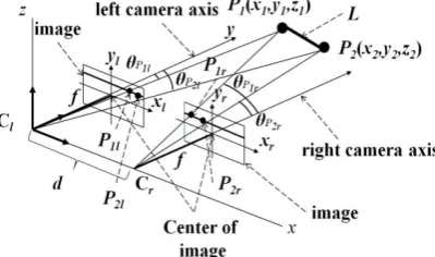
The basic concept of survey-from-photo is that of the "stereo vision" principle, which uses two cameras to measure dimensions of an object, as presented in Figure 2. One camera is located at Cr and another at Cl with intervening distance (d). The cameras are focused at point P1(x1, y1, z1) and P2(x2, y2, z2) with certain focus length (f),

which are all obtainable at the camera lens. At f, two image points are apparent at the image P1r, P1l, P2r, and P2l with respective coordinates (x1r,y1r), (x1l,y1l), (x2r,y2r), and

(x2l,y2l). The coordinates (x1r,y1r), (x1l,y1l), (x2r,y2r), and (x2l,y2l) are calculable by

considering the center of image as the origin. To obtain the coordinate of P1(x1,y1,z1)

and P2(x2,y2,z2), the equation is definable simply as shown below.

(1)

(2)

Lx=d

x_1l x₁l-x1r

- x2l

x₂l-x2r

æ è

ç ö

ø

÷ (3)

L_y=d y1l

x_1l-x_1r -y_2l x_2l-x₂r æ

è

ç ö

ø

÷ (4)

Lz =df

1 x₂l-x2r

- 1

x₂l-x2r

æ è

ç ö

ø

÷ (5)

The distance (L) between P1 and P2 can be simplified as;

L= L_x2+_L

y

2+_L

z

2

(6)

iii. Neural Network (NN)

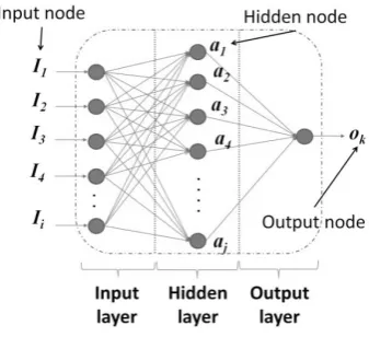
Basically, NN architecture involves three layers; input layer, hidden layer and output layer. Each layer consists of number of nodes to construct a network connection as shown in Figure 3. Detail explanation of NN can be referred to previous paper (Yahya, M.N, et. al., 2010).

5

randomly. To obtain the optimum network, 2–15 hidden nodes are used. The mean square error (MSE) and correlation coefficients (r) are used for assessment.

Figure 3: Architecture of NN

METHODOLOGY OF SUBSYSTEM_1

i. Material Surface Capturing

For this study, six material surfaces were taken of Oita University rooms, as portrayed in Figure 4. Surfaces (a), (b), (c), (d), (e), and (f) are, respectively, surfaces for walls, doors, floors, windows, ceilings, and carpets. To perform material surfaces capturing, an ordinary camera is useful. Regarding standardization of images, a digital single-lens reflex (DSLR) camera with Sigma 50 mm f2.8 lens was used. In addition, the distance from the camera to the surface material was set to 40 mm with autofocus mode, whereas the respective lens settings for aperture, shutter speed and ISO speed were f2.8, 1/80, and 100. To analyze the accuracy of Subsystem 1, 368 images of surfaces were captured at different locations in three rooms. The proportions of images of material surfaces are: surface (a) = 69 images, surface (b) =71 images, surface (c) = 66 images, surface (d) = 56 images, surface (e) = 67 images, and surface (f) = 40 images. All images were analyzed using GLCM.

Figure 4: Sample images of material surfaces for (a) wall, (b) door, (c) floor, (d) window (e) ceilling and (f) carpet

ii. GLCM Implementation

(d) (e) (f)

6

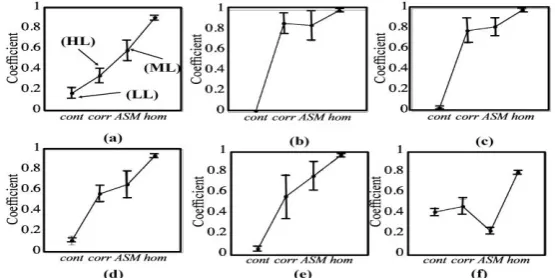
The GLCM was computed for the 368 images of surface materials using the following settings: i. d = 1, θ = 0°; ii. d = 1, θ = 45°; iii. d = 1, θ = 90°; and iv. d = 1, θ = 135°. Each Haralick's coefficient provides four values based on settings, but only an average value of four values is considered hereinafter. The average value is designated as the coefficient value for this study. Because of variations of brightness and texture features in our experiment, the ranges of the coefficient values become too wide to be processed. To overcome this problem, a limitation for each coefficient value was made using the means (x) and standard deviation (σ). The limitations are (x ˗ σ) and (x + σ), respectively, for low limitation and high limitation. The coefficient values beyond the limitations were removed from further investigation.

iii. FFNN Implementation

Coefficient values in the limitation were fed into NN. Four coefficients (cont,

corr, ASM, and hom) and the material surface were used respectively as input nodes and output nodes. Then the numbers of hidden nodes were set up as described previously. In addition, the learning algorithm chosen was Levenberg–Marquardt (trainlm) because it is faster and more efficient). To obtain the optimum network, a trial and error scheme was conducted by combining all those nodes (e.g. [i; h; o] for [input node; hidden node; output node]; example combination [4, 6, 1], [4,10,1], … or [4, 9, 1]) but only one combination that provided good performance was selected.

METHODOLOGY OF SUBSYSTEM_2

i. DVP Implementation

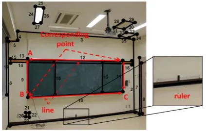
The same camera for Subsystem_1 was used with focus lenses of 18–70 mm to capture two images at one view. The camera was set in autofocus mode. Figure 5

presents an example of predicting dimensions of objects in one image at one view. Lines connect corresponding points at objects. For example, to measure blackboard object dimensions, four corresponding points of A, B, C, and D must be obtained. Each corresponding point is connected to form lines: line 9, 10, 11, and 12. As described above, the survey-from-photo requires a standard scale. Therefore, the authors propose to use a ruler that is attached at an appropriate view as reference dimension in this "ruler method". A ruler is preferred because it is practical and simple to attach to the view region to be measured.

7

Figure 5: Identification dimension

METHODOLOGY OF SYSTEM

i. FEA Implementation

To obtain the RTs database of rooms which are used for construction of NN, 20 rooms with different volumes were simulated using FEA. In simulation, six absorption coefficients of surface materials at wall, door, window, floor, ceiling and furniture were considered in this study. Basically, the absorption coefficient values (ranging 0 to 1) are depending on the type of material either reflective or absorptive. To consider all the absorption coefficient values, it will increase the computing time and cost of FEA. To overcome the problem, two kind of conditions were considered; i. dead: (α_w = 0.08; α_dr = 0.1; α_wdw = 0.4; α_flr = 0.06; α_clg = 0.4; α_f = 0.4 ); ii. live: (α_w = 0.02; α_dr = 0.02; α_wdw = 0.04; α_flr = 0.02; α_clg = 0.2; α_f = 0.4), where α_w, α_dr, α_wdw, α_flr, α_clg, and α_f representing absorption coefficient for wall, door, window, floor, ceiling and furniture, respectively. Dead is the maximum value of absorption coefficient, whereas live is the minimum value of absorption coefficient. These conditions were obtained from several surface materials at Oita University's room. Furthermore, another 6 rooms were simulated using FEA. These rooms were used to test the performance of NN.

ii. NN Implementation

Database of 1220 RTs obtained from 20 simulated rooms by FEA were fed into NN. The database was divided into two subsets one is train subset (70% of database) and the other is validate subset (30% of database). To confirm the reliability of prediction, the 360 testing database of RTs obtained from the six simulated rooms were involved.

RESULTS AND DISCUSSION

i. Subsystem_1

8

images of surfaces (surface (a) = 39 images, surface (b) = 50 images, surface (c) = 27 images, surface (d) = 26 images, surface (e) = 30 images, and surface (f) = 20 images) were used for NN as input nodes because of limitations. Before feeding into NN, a database of images of surface materials was divided into three subsets: 60% of the database for training; 20% of the database for validation, and 20% of the database for testing. No specific proportions for NN subsets were set. At this point, the proportions of subsets are chosen arbitrarily. Generally, the training subset should be larger than the validation subset and the testing subset.

Figure 6: Limitation of coefficient values for six material

In this study, the absorption coefficients (α) of six material surfaces are referred from reports of the relevant literature (Maekawa and Lord, 1993). By identifying the material surfaces, we are able to ascertain the absorption coefficients of surfaces simultaneously. To identify the material surfaces, we used a classification number (1–5) to represent the output parameter: 1. Surface (a) (α = 0.07), 2. Surface (b) and (c) (α = 0.02), 3. Surface (d) (α = 0.04), 4. Surface (e) (α = 0.4) and 5. Surface (f) (α = 0.06).

Results of analyses show that the optimum network [4, 6, 1] with MSE ≤ 0.0018 and r ≥ 0.9 was obtained for both training and validation subsets. To confirm their performance, the testing subset (39 surface images) showed MSE ≤ 0.07 with r ≥ 0.9. Subsystem_1 performance is inferred to be good at this stage.

The restrictions of Subsystem_1 are the following: 1. It can only identify the material surfaces depending on the database of material surfaces used. If more databases of material surfaces were used, then more material surfaces can be identified. 2. Generally, the real absorption coefficients of material surfaces in rooms depend on the material thickness, presence or absence of an air layer and absorptive layer, and so on. Then, it is difficult to obtain a real absorption coefficient only a surface form image. For practical usage, the author referred to related reports of the absorption coefficient.

ii. Subsystem_2

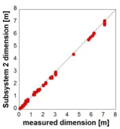
From analyses of Subsystem_2, the results are given in Figure 7, which revealed a high correlation coefficient (r ≥ 0.99) between predicted values using Subsystem_2 and measured values with MSE ≤ 0.009. Results show that Subsystem 2 provided high reliability using no physical measurements.

9

From the analysis, the optimum network is [4,11,1] with train and validate database indicate MSE ≤ 0.0012 with r ≥ 0.9 for both of them. Furthermore, for confirmation the testing database indicated MSE ≤ 0.007 and r ≥ 0.80. At this point, the NN that used for System are developed. It gives good reliability of prediction RTs on six simulated rooms.

iv. Implementation at actual room

Four types of actual rooms were utilized to investigate the predicting reliability of Sub-systems and System. At Sub-system-1, the 294 surface images (surface (a) = 60 surface images, surface (b) = 53 surface images, surface (c) = 48 surface images, surface (d) = 63 surface images, surface (e) = 41 surface images and surface (f) = 25 surface images) were captured. However, only 180 surface images were selected after normalization (x). These surface images were fed into NN. At Sub-system-2, the target objects were room, door, window and furniture (desk and chair). These objects were captured and fed into DVP to predict the dimensions. Later on, predictions from both Sub-systems were moved to the System using NN. Besides that, the prediction from Systems_1 and Subsystem_2 also moved to FEA. The prediction reliability of RT using System and FEA were examined.

Figure 8 reveals that prediction by Subsystem_1 which gives high r ≥ 0.9. Unfortunately, predictions on 3 (Surface (d): window (α = 0.04)) showed inconsistent results. It is because 29% of 31 surface images indicated below limit at ASM. The window is a transparent and lighting reflection material. In this case of the transparent window, it is difficult to capture consistent surface images due to the material surface nature.

Figure 9 shows the prediction results of dimension of room. Following the capturing procedure, the DVP produce high r ≥ 0.9 in predicting the dimensions.

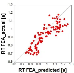
To predict RTs, the System (using NN) and FEA used same input parameters obtained from Subsystem_1 and Subsystem_2. The System provided inconsistent prediction with between FEA. On the other hand, by using the actual input parameter obtained from four rooms the FEA gave a consistent prediction. Figure 10 depicts the correlation between FEA actual and FEA predicted is more than 0.80. From the observation, at the moment, the technique in Subsystem_1 and Subsystem_2 provided good prediction reliability when there are utilized with FEA.

10

CONCLUSION

Aiming for practical application prediction technique of absorption coefficient and dimension using photographic image and NN were developed. In Subsystem_1 consists of GLCM and NN to predict the absorption coefficient. While in Subsystem_2 consists of DVP to predict the dimension. The result from Subsystem_1 and Subsystem_2 show good reliability with r > 0.9. The System and FEA are used to predict RTs. By the comparison between them, it shows that FEA offer more consistent result with the r 0.8. From the averall results, we can concluded that by applying the Subsystem_1 and System 2, the practical value of absorption coefficeint and dimension could be predicted. At this stage, the predicted value from Subsystem_1 and Subsystem_2 are useful to predict the RTs of room by using the consistent method such as FEA, BEM, and Empirical Method

ACKNOWLEDGEMENT

This study is supported by RAGS (KPT) grant – R014 which are managed by Research, Inovation, Commercialization and Consultancy Office (ORICC), UTHM.

REFERENCES

Hodgson, M. 2009. Ray-Tracing prediction of optimal conditions for speech in realistic classrooms. Applied Acoustics, 70: 915-920

Okuzono, T. 2010. Fundamental accuracy of time domain finite element method for sound-field analysis of rooms. Applied Acoustics, 71(10): 1027-1067

Hodgson, M. 2005. Estimate of the absorption coefficients of the surfaces of classrooms. Applied Acoustics 67: 936-944

Honneycutt, C.E. and Plotnick, R. 2008. Image Analysis Techniques and Gray-Level Co-occurrence Matrices (GLCM) for calcultaing bioturbantion indices and characteristic biogenic sedimentary structure. Computer & Geoscience. 34: 1461-1472

Haralick, R.M, Shanmugam, K and Disntein, I. 1973. Textural features for image classification. IEEE Transaction System. 3: 610-621

Musli Nizam Yahya, Otsuru. T, Tomiku, R. and Okuzono, T. 2010. Ivestigation the Capability of Neural Network in Predicting Reverberation Time on Classroom. International Journal of Sustainable Construction Engineering & Technology. 19-31

Maekawa, Z. and Lord, P. 1993. Enviromental and Architectural Acoustics. E&FN Spon

Figure 9: Correlation for Subsystem_2