Methods in Computational Protein Design

Thesis by Victor Wai Tak Kam

In Partial Fulfillment of the Requirements for the degree of

Doctor of Philosophy

CALIFORNIA INSTITUTE OF TECHNOLOGY

Pasadena, California 2008

© 2008

Acknowledgements

I dedicate this thesis to my parents. Without all their support and encouragement, I would not even be here writing this.

Getting a Ph.D. is hard. But it was enjoyable when you are given the freedom to explore problems from directions of your choice. I thank my advisor, Professor Bill Goddard, for the support and faith he entrusted in me. I have much to learn from him—the creativity he displays towards solving problems, the breadth and depth of his knowledge, and his boundless energy and enthusiasm. I would also like to thank Dr. Vaidehi Nagarajan, who put in an enormous amount of time and effort and has always been a great friend.

Abstract

In silico design of protein has generated enormous interest with the rapid advances in computational power. Biological systems are known for their complexity, and we have made a series of computational developments that allow us to perform computational protein design. In this work we present a methodology for the design and prediction of protein active sites.

We begin by presenting SCREAM, a program developed to accurately position sidechains in proteins. We show how using an improved scoring function and placement algorithm allow us to achieve better accuracy in the placement and prediction of sidechains in proteins compared to other methods.

We then describe the development of an accurate treatment for describing hydrogen bonding. This is done by refining the hydrogen bond term in the force field DREIDING. We also need to properly describe electrostatics effects in proteins, and to this end, we introduce neutralized residues for proteins. We found that this improves the variance in our predictions dramatically.

Table of Contents

Acknowledgements...iii

Abstract... 1

Table of Contents ... 2

1 Computational Protein Design: Overview... 14

1.1 Protein Sidechain Conformation Search... 14

1.1.1 Rotamers... 15

1.1.2 Placement of Sidechains... 16

1.2 Energy Expressions... 16

1.2.1 Covalent Terms ... 17

1.2.2 Non-covalent Terms ... 18

1.3 Summary ... 20

2 SCREAM ... 21

2.1 Introduction... 21

2.2 Materials and Methods... 22

2.2.1 Preparation of Rotamer Libraries... 22

2.2.2 Preparation of Structures for Validation of SCREAM... 23

2.2.3 Surface Area Calculations ... 25

2.2.4 Positioning of Sidechains ... 25

2.2.5 Combinatorial Placement Algorithm... 25

2.2.6 The Flat-Bottom Scoring Function... 28

2.3 Results and Discussion ... 34

2.3.1 Single Placement of Side-chains... 34

2.3.2 Effects of Buried vs. Exposed Residues ... 37

2.3.4 Analysis of Impact of Flat-Bottom on Individual Amino Acids during Combinatorial

Placement ... 42

2.3.5 Effects of Minimization on Structures from Different Scaling Factors ... 42

2.3.6 Program Execution Performance ... 45

2.3.7 Tests on the Liang Set Using the Optimized Scaling Factor... 46

2.3.8 Parameters for Other Lennard Jones Potentials... 47

2.3.9 Comparison with VDW Radii Scaling... 48

2.3.10 Extension beyond the Natural Amino Acids... 49

2.4 Conclusion... 49

3 DREIDING for Polar Interactions ... 50

3.1 Introduction... 50

3.2 Polar Interactions ... 51

3.2.1 Neutralizing Amino Acids... 51

3.2.2 Assignment of Protons from Neutralization of Charged Residues ... 53

3.3 DREIDING Hydrogen Bond Term... 55

3.3.1 Introduction... 55

3.3.2 Updating the DREIDING Hydrogen Bond Term ... 56

3.4 Optimization of Hydrogen Bond Parameters... 64

3.4.1 Atom Types for Hydrogen Bond Donors and Acceptors... 64

3.4.2 VDW Parameters... 66

3.4.3 Hydrogen Bond Parameterization Methodology ... 67

3.4.4 Parameterization of Neutral Hydrogen Bond Atom Types... 69

3.4.5 Parameterization for Neutralized Form of Charged Residues... 72

3.4.6 Validation ... 73

3.5 Applications... 75

3.5.1 Protein Structure Preparation... 75

3.5.2 Effect on Molecular Dynamics: An Example... 78

3.5.3 Bovine Rhodopsin Helical bundle... 83

3.6 Conclusion... 87

4.1 Introduction... 88

4.1.1 Methods and Material ... 88

4.1.2 The Design Protocol—Energy Excitation... 89

4.2 Design of Human Inteferon-β... 96

4.2.1 Introduction... 96

4.2.2 Single Mutations... 96

4.2.3 Combinatorial Mutations of Residues around Met 62... 99

4.3 Active Site Design of TrpRS ... 101

4.3.1 Introduction... 101

4.3.2 Bacillus Stearothermophilus TrpRS Active Site Design ... 105

4.3.3 Human TrpRS Active Site Design ... 111

Appendix A SCREAM Supplementary Material... 125

A.1 Prediction of Surface Residues Prior to Sidechain Assignment ... 125

A.2 Impact of Scaling Factor s in Combinatorial Placement: ... 126

Appendix B Algorithms Used in Neutralizing Residues... 132

B.1 Flow Network ... 132

B.2 Remark on Correctness ... 134

LIST OF ILLUSTRATIONS

Figure 1-1 Illustration of 2 rotamers of the amino acid glutamine...15 Figure 2-1 The flat-bottom potential. The inner wall is shifted by an amount Δ. ...29 Figure 2-2 Effects on dielectric value on RMSD. The optimum value for the constant

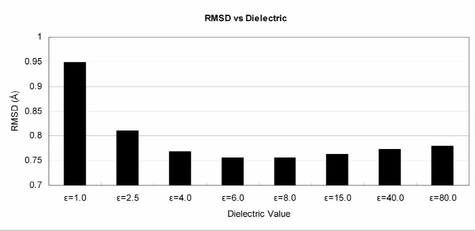
dielectric, ε=6.0 shown here, was obtained by fitting results for the Xiang set with a diversity of 1.0Å and a scaling factor s of 1.0. ...33 Figure 2-3 Single sidechain placement accuracy for various rotamer libraries at different s

values. Shown are the libraries of 0.2Å diversity (14755 rotamers), 0.6Å diversity (3195 rotamers), 1.0Å diversity (1014 rotamers), 1.4Å diversity (378 rotamers), 1.8Å diversity (218) and all-torsion (382 rotamers). The coarser the rotamer library is, the more pronounced the effect of s becomes...35 Figure 2-4 The effects of varying the scaling factor s on placement accuracies for the

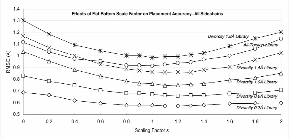
exposed and core residues. Shown are results from the 1.4Å diversity rotamer library results. Exposed residues account for approximately 25% of all residues..38 Figure 2-5 Accuracy for simultaneously replacing all sidechains for various rotamer

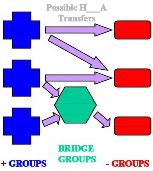
libraries at different s values. Shown are the libraries of 0.6Å diversity (3195 rotamers), 1.0Å diversity (1014 rotamers), 1.4Å diversity (378 rotamers), 1.8Å diversity (218) and all-torsion (382 rotamers)...40 Figure 3-1 The four charged amino acids at physiological pH...51 Figure 3-2 Schematic illustrating the movement and assignment of protons. Arrows

denote possible polar hydrogen “+ Groups”: functional groups that are positively charged, i.e. those with extra protons. “- Groups”: functional groups that are negatively charged, i.e. those that can accept protons. “Bridge Groups”: groups such as H20 or Histidine that can form hydrogen bonds between + Groups and –

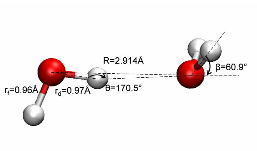
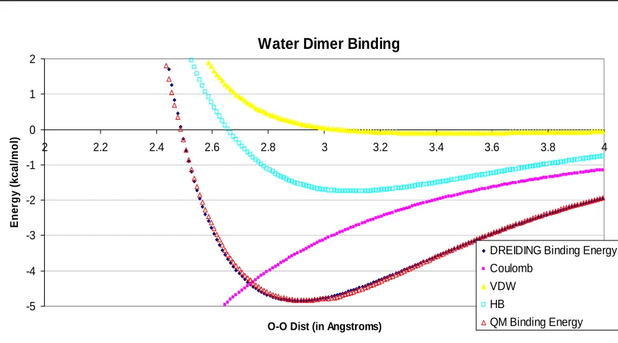
Figure 3-4 Water dimer binding, QM vs. DREIDING using fitted parameters with a Morse hydrogen bond potential with γ=9.70, R0=3.10 and D0=1.75. ...60

Figure 3-5 Angle dependence of water dimer binding. Note that the angle shown here is the O…O-H angle, not the O-H…O angle in θAHD. ...62

Figure 3-6 Samll molecule model compounds used in parameterization of hydrogen bonds common in proteins. ...67 Figure 3-7 Small molecule model compounds for neutralized form of charged amino acids.68 Figure 3-8 The 14 small molecules chosen in our test set...74 Figure 3-9 A salt bridge pair that was minimized into existence using charged residues.

The protein shown is 1isu. Shown are the final minimized structure of the charged protein, neutralized protein, and the initial crystal structure of the residues Lysine 17 and Aspartate 56. ...78 Figure 3-10 RMSD of protein heavy atoms for a charged and a neutral system, compared

to initial simulation structure. 500 ps of simulation is shown...80 Figure 3-11 Residue R27 and E29 in IFN-β. The two residues are 3.7Ǻ apart in the initial

structure. ...81 Figure 3-12 Evolution of distance between Cδ atom of E29 and Cζ atom on R27. ...81 Figure 3-13 Residue R152 and E149 in IFN-β. The two residues are 4.3Ǻ apart in the

initial structure...82 Figure 3-14 Evolution of distance between Cδ atom of E149 and Cζ atom on R152. ...82 Figure 3-15 Top-down view of a GPCR with its 7 helixes. Each rotational axis of a helix

is defined according to the MembStruk protocol...84 Figure 4-1 Flowchart for introducing mutations by using the “Singles Excitation” strategy.90 Figure 4-2 Human IFN-β (pdb code: 1au1). Methionines are shown in ball and stick

format. Met 36 is the one on the bottom left hand corner, Met 117 top left hand corner, Met 62 the one positioned in the middle. Distances between the

Figure 4-3 Residues near position 62 in human IFN-β. Ile40 and Ile44 are identified as residues that are in direct contact with Met62 and needs to be mutated when

changes to Met62 is made. ...100 Figure 4-4 Cartoon depicting the role played by an amino-acyl tRNA synthetase. The

amino acid tryptophan is being charged in this example. (Adapted from Ibba. et al79)...102 Figure 4-5 Illustration of an uncatalzyed azide-alkyne 1,3-cycloaddition...103 Figure 4-6 Non-natural amino acid analogs of Trptophan with functional groups that are

relevant to click chemistry. ...104 Figure 4-7 The active site of B. Stearothermophilus TrpRS with cognate Trp ligand. The

ligand is shown in licorice representation, whereas the residues interacting with the ligand is shown in ball-and-stick format. ...106 Figure 4-8 The active site of B. Stearothermophilus TrpRS with 5-ethynyl-Trp ligand. The ligand is shown in licorice representation. V141 and V143, two residues potentially interacting with the ligand, are shown in ball-and-stick format. ...107 Figure 4-9 Residues around D132 in B. Stearothermophilus TrpRS. One of the oxygens of

D132 serves as the hydrogen bond acceptor of the HN group of Trp. ...110 Figure 4-10 Binding site of human TrpRS (pdb code 2dr2). Cys309 and Ile307 can be

mutated to accommodate larger ligand in the binding pocket...113 Figure 4-11 Binding site of 2dr2 with indene amino acid analog and top mutation

candidates at positions 159, 194 and 237. ...114 Figure 4-12 Two possible configurations for the oxyethynyl groups...116 Figure 4-13 Starting configuration for the unnatural amino acid analog propargyloxy-Trp.

The ethynyl group is off the Trp ring plane by 60°...118 Figure 4-14 Top mutation candidate for propargyloxy-Trp as ligand in human TrpRS...119 Figure 4-15 Homoazido-Trp as ligand. Clashes with C309 and I307 are shown...120 Figure 4-16 Possible configurations of benzo-cyclo-octyne amion acid analog...121 Figure 4-17 Three out of four possible configurations of benzo-cyclo-octyne amino acid

LIST OF TABLES

Table 2-1 Number of rotamers in libraries of various diversities. ...23 Table 2-2 δ and σ values for each atom on the Arginine side-chain, listed in order of

distance away from the mainchain. Nη1 and Nη2 are equivalent atoms; the average value is used in actual calculations. These numbers were obtained from the rotamer library of diversity 1.0Ǻ...30 Table 2-3 δ and σ values for each atom on the Lysine side-chain, listed in order of distance

away from the mainchain. These numbers were obtained from the rotamer library of diversity 1.0Ǻ...30 Table 2-4 Optimized s value for rotamer libraries of size ranging from 0.2Å to 5.0Å, plus

the all torsion rotamer library. The s values that give the best RMSD value are listed ...36 Table 2-5 Effect of s values on χ1/χ1+2 accuracy. Rotamer libraries of diversity ranging

from 0.2Å to 5.0Å, plus the all torsion rotamer library are used. The best χ1+2 accuracy is used to determine the most effective scaling factor s. A χ angle is considered correct if within 40∘of the corresponding χ angle in the crystal sidechain conformation. ...37 Table 2-6 Accuracy comparison in single sidechain placements for buried and exposed

residues for the Xiang test set...39 Table 2-7 Optimized s value for rotamer libraries of size ranging from 0.2Å to 5.0Å, plus

the all torsion rotamer library. The scaling factor s that gives the best RMSD value is included. For comparison, SCWRL gives a RMSD of 0.95Å for the same

Table 2-8 Effect of s values on χ1/χ1+2 accuracy. Rotamer libraries of diversity ranging from 0.2Å to 5.0Å, plus the all torsion rotamer library are used. The best value for

χ1+2 correctness is used to determine the most effective s value. A χ angle is considered correct if within 40° of the corresponding χ angle in the crystal

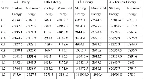
sidechain conformation. The χ1/χ1+2 correctness for SCWRL is 86.4% / 79.7%. 42 Table 2-9 Average energy values for the 33 proteins over varying s values. All energy

values include valence and non-valence terms, and the units are presented in kcal/mol. The energies do not include interaction terms between atoms that are not involved in the sidechain placement calculations. Numbers in bold are the

minimum values for each category. ...44 Table 2-10 Average RMSD values (in Å) for the Xiang set of 33 proteins, before and after

minimization. Entries in bold correspond to those with the lowest DREIDING energies before and after minimization, see Table 2-9 for details...45 Table 2-11 Performance measure of SCREAM, with rotamer libraries of various

diversities. The timing statistics were taken from the runs that gave the best energy values...46 Table 2-12 SCREAM predictions on the Liang test set using optimized scaling factor for

rotamer libraries of various diversities. The percentage of buried residues in this test set is about 40%, greater than the 25% figure from the previous test set. We include crystal structure solvents in the predictions, and the increase in exposed residues is due to the fewer resolved solvents in those structures...47 Table 2-13 Effect of different Lennard-Jones potentials and their optimal scaling factor s.

Tests were done on the Xiang protein set using the 1.0Ǻ rotamer library...48 Table 2-14 Effects of VDW scaling. Tests were done on the Xiang protein set using the

1.0Ǻ rotamer library...49 Table 3-1 Interaction energies of model charged compounds (see Figure 3-7) representing

Table 3-2 New atom subtypes for atoms on previously charged residues. The suffixes “M” and “P” at the end of a neutralized atom type stand for “Minus” and “Plus”,

mnemonics for remembering the original net charge of the residue the atom belongs to. For ASP and GLU, the atom type O_3M is used on the oxygen with a proton added onto it...55 Table 3-3 Mulliken charges for water, when using different basis sets. Except for the

6-31G basis set, where the Hartree-Fock method is used, all other calculations are done using the X3LYP method. The dipole moment is calculated by placing the charges on water molecule atoms. ...58 Table 3-4 DREIDING atom types for oxygen (O_3W) and hydrogen (H___A) in water.

Mulliken charges for the water monomer are based on calculations at the X3LYP/aug-cc-pvtz(-f) level. The R0 off-diagonal O_3 – H___A term is the

geometric mean of the two R0 values for H___A and O_3...59

Table 3-5 Comparison of binding energies of water dimers in various water models. Final minimized values are reported...63 Table 3-6 DREIDING atoms types that are used in proteins. (1): Amide was picked

because ethers do not naturally occur in proteins...66 Table 3-7 Off-diagonal VDW terms for hydrogen bond acceptors and the hydrogen

bonding hydrogen (H___A). R0 values are derived from geometric mean of heavy

atom VDW radii and H___A VDW radii...66 Table 3-8 (continued) Fitting parameters for all atom types that are present in neutral

residues in proteins. The accuracy fitting is within 0.1kcal/mol in overall binding energies and 0.1Ǻ in the equilibrium distance between hydrogen bond donor and acceptor atoms. Me-Im: Methyl Imidazole at the delta position, CH3C3H4N2.

Amide: Methyl-Amide, CH3CONH2. (1) Involves two hydrogen bonds. (2)No

hydrogen bond term necessary, since electrostatics is sufficient to account for the polar interaction...72 Table 3-9 Fitted parameters for interaction between salt bridges, allowing for proton

Table 3-10 Average error in force field binding energies and donor/acceptor distances

compared to quantum mechanics for the test set of 20 hydrogen bond forming pairs.75 Table 3-11 RMSD comparison of minimization of charged and neutralized proteins to

original crystal coordinates. ...77 Table 3-12 Top ranking structures using energies from neutralized system. The helix

rotated is indicated in the second character, and the degree of rotation is indicated by the final 3 characters. Overall energy includes all valence terms and

non-valence terms...86 Table 3-13 Top Ranking structures using energies from the charged system...86 Table 4-1 Internal energies, experimental solvation energies and surface area for each of

the 20 amino acids. ...93 Table 4-2 Energies for top mutations introduced at position 36 of human IFN-β. Energy

values are relative to the wildtype Methionine energy. ...97 Table 4-3 Energies for top mutations introduced at position 117 of human IFN-β. Energy

values are relative to the wildtype Methionine energy. ...98 Table 4-4 Top mutation candidates introduced at position 62 of human IFN-β. ...99 Table 4-5 Energies for various mutations in the hydrophobic pocket around Met 62. The

wildtype energy is used as reference for other mutations...99 Table 4-6 Interaction energies for single mutations at position 143 in the presence of

5-Ethynyl Trp in place of cognate Trp ligand. The energy of the best mutation is used as a reference energy...107 Table 4-7 Binding energies and differential binding of V143A and V143G mutations of

5-Ethynyl-Trp compared to the cognate Trp ligand. ...108 Table 4-8 Mutation at position 132 of B. Stearothermophilus TrpRS. The indole ring of the cognate Trp ligand has been replaced by an indene ring. ...109 Table 4-9 Double mutations at position 132 and 80 of B. Stearothermophilus TrpRS. ...111 Table 4-10 Top mutation candidates for positions 159, 194 and 237 when the ligand in

Table 4-11 Binding energy of cognate ligand and indene analog with top mutation

1

Computational Protein Design: Overview

Protein design is becoming a practical option for solving problems in protein engineering. The growth in this field has been greatly facilitated by the rapid increase in computational prowess and algorithmic advances made in the past two decades, and investigations today address a wide variety of problems. Progress is not only limited to academic researchers, but also to the industry, as computational methods are gradually being accepted as part of the drug discovery process. The permeation of computational methodologies is certain to continue as pharmaceutical companies face growing pressure to reduce development costs of new drugs, estimated at over $800 million1 _{as of 2006.}

Computational protein design is the process of introducing mutations in the original sequence of a target protein in order to introduce desired properties through computational means. Examples include improving stability between protein-protein interactions2 and mutation of an active site of a protein to incorporate a non-cognate ligand3. There are two major difficulties with regards to introducing mutations. The first is how to predict

computationally the positioning of other sidechains or atoms after the mutations, a problem known as the conformation search problem. The second is how to accurately assess the favorability of the mutations introduced, known as the energy function problem.

1.1

Protein Sidechain Conformation Search

the input, either from the crystal structure of the protein, from homology modeling, or from other ab initio methods.

The assumption of a known protein backbone simplifies the search problem considerably, but the search space is still huge. There are 20 possible amino acids for each residue, and each amino acid sidechain have multiple conformations. The sheer number of

combinations is huge. Consider the following. If each amino acid sidechain can take on 5 possible conformations, each amino acid can have 5 possible mutations, and there are 100 possible sites on the protein, then there are a total of 5100·5100 ≈10280 possibilities! This number is greater than the number of atoms in the universe and certainly not tractable by any computational means. Fortunately, many of these possibilities can be eliminated quickly and it is possible to arrive at reliable conformations by using various methods, procedures and algorithms4-9 that have been developed in the past two decades.

1.1.1 Rotamers

Instead of working in the continuous conformational search space when placing amino acid sidechains on the protein backbone, Ponders and Richards10 introduced using discrete sidechains configurations that occur frequently in protein structures. These low-energy conformations are called “rotamers” (see Figure 1-1 for two rotamers of the glutamine sidechain), short for rotational isomers.

OO

2 rotamers of

2 rotamers of

glutamine

glutamine

O O

2 rotamers of

2 rotamers of

glutamine

glutamine

Each amino acid sidechain needs to be represented by a number of these rotamers. For amino acids such as arginine and lysine that have more torsional freedoms, more rotamers are needed to cover the conformation space. Conversely, simpler amino acids such as serine only need a small number of rotamers. A collection of rotamers that represent the amino acids is called a rotamer library5,11. The structures of the rotamers can be taken from crystal structures in proteins or be constructed according to chemical principles, such as energy minima of torsional angles. Clearly, the more rotamers we use, the more complete the rotational search space we are sampling and more accurate the results, but at an

increased performance cost. Therefore, there is a trade-off between the accuracy (more rotamers) and speed (fewer rotamers) in our search problem. In Chapter 2, we explore methods to reduce the cost of the trade-off.

1.1.2 Placement of Sidechains

After we place the rotamers onto the protein backbone, we need to decide which

configurations are better than others. This is done by using a scoring function8, which can be energy-based, statistics-based, or some combination of the two. After deciding on a scoring function, there is also the global optimization problem of finding the combination of rotamers that yield the best score given the scoring function. Because of the

combinatorial nature of the problem, a brute-force search will not be successful in finding a good solution to this problem. Many approaches have been developed12_.

In Chapter 2, we go into more details on energy-based scoring functions and a mean-field approach to the placement of sidechains.

1.2

Energy Expressions

including simulation of large biomolecules, the level of information obtained from quantum mechanics is unnecessary.

Molecular mechanical force fields13,14 _{have been developed to perform accurate}

calculations in a more reasonable amount of time. These force fields use simpler energy expressions to describe interactions between molecules, and are parameterized against experimental or quantum mechanical calculations. Popular force fields in the study of biological systems include CHARMM13, AMBER15 and DREIDING14. The accuracy of these force fields allows the study of such complex problems in molecular biology such as protein folding16,17, molecular docking18, and ab initio structure prediction19,20. Indeed, many commercial software, such as Accelrys’ Quanta and Cerius2, include these biological force fields in the distribution.

We briefly review components of a biological force field. The total overall energy of a system is divided into valence terms and non-valence terms:

E = E

+ E

In the following section, we describe the functional forms that are used in DREIDING. Similar functions are used for other force fields.

1.2.1 Covalent Terms

DREIDING divides the valence terms into four components:

E

= E

+ E

+ E

+ E

where Eb is the bond stretch energy between two atoms, Ea the bond angle energy between

three atoms, Et the torsional angle energy between four atoms, and Ei the inversion term

between four atoms. For Eb, Ea and Et, a harmonic expression is often employed to capture

values, for these terms are parameterized. Ei, the inversion term, is a special term in

DREIDING that ensures the molecules stay planar (as in benzene) or maintain the correct chirality during simulations. A harmonic expression can also be used here.

Valence bonds are never broken in DREIDING and most other biological force fields.

1.2.2 Non-covalent Terms

Many interesting phenomena in bio-molecules involve non-covalent interaction between molecules, such as a ligand binding to a receptor. Thus, the accurate description between non-bonded atoms is crucial to the accurate prediction of inter-molecular properties such as binding energies. In DREIDING, non-valence terms include:

E

=

E

+ E

+ E

where EVDW is the two-body van der Waals (VDW) energy (also known as dispersion), EQ

the two-body Coulombic or electrostatic interaction, and EHB a special three-body hydrogen

bond term.

Historically, the Lennard-Jones 12-6 potential is often used as the expression for the VDW term:

]

)

/

(

2

)

/

[(

)

(

R

D

R

R

R

R

E

=

−

where DVDW is the equilibrium VDW well-depth of a pair of atoms, RVDW the equilibrium

asymptotic behavior at large distances, reflecting the fact that its origin lies in the instantaneous but fluctuating dipole moments of neutral atoms.

Typically, the equilibrium radial distance between two atoms is the sum of the atomic radii of the two interacting atoms. There are instances when we do not want this, and we will show an example in Chapter 3.

The classic Coulomb interaction form is used for the electrostatic term:

ij j i

Q

Q

Q

R

E

=

(

322

.

0637

)

/

ε

where the energy is expressed in kcal/mol and Rij is expressed in Ǻ. Qi, Qjare point

charges assigned to center of atoms. The dielectric constant is usually taken to be ε=1.0, but values greater than 1.0 have been used to account for the effect of polarization. We go into more detail on this issue in Chapter 3.

DREIDING uses a 3-body hydrogen bond term that is not common in many other force fields:

)

(

cos

]

)

/

(

6

)

/

(

5

[

DHA DA hb DA hb hb

hb

D

R

R

R

R

E

=

−

θ

where Dhb stands for the well-depth of the hydrogen bond potential, Rhb the equilibrium

distance and θDHA the angle between the hydrogen bond donor atom, hydrogen and the

component of bio-molecular recognition, we explore different hydrogen bond functions in Chapter 3 in an effort to improve the accuracy.

1.3

Summary

2

SCREAM

2.1

Introduction

In developing general predictive approaches for structures of membrane proteins21-23_{, we}

found that current available sidechain placement methods, e.g. SCWRL, did not provide sufficiently accurate results to determine the helix-helix relative orientations within the membrane. Consequently, we developed the SCREAM (SideChain Rotamer Energy Analysis Methodology) approach reported here, which we have found to lead to

dramatically improved protein structures. Here, we present validation of SCREAM against standard libraries of crystal structures.

As briefly mentioned in Chapter 1, sidechain placement methods play a major role in recent applications in the field of computational molecular biology; from protein design24-26, flexible ligand docking27, loop-building28, to prediction of protein structures29. Much attention has been paid to this important problem, which is difficult because it is in a category of problems known as NP-hard30, for which no efficient algorithm is known to exist. Since the groundbreaking work by Ponder and Richards10, many approaches have been developed, including mean-field approximation6,31, Monte Carlo algorithms7,32, and Dead-End Elimination (DEE)4,33-35. In practice, however, studies have also concluded that the combinatorial issue may not be as severe as originally thought36,37. Compared to the placement methods and rotamer libraries, scoring functions have not been studied as extensively8,38,39. Here, we focus on the scoring function.

Our scoring function is based on the all-atom forcefield DREIDING14 _{which includes an}

explicit hydrogen bond term. The use of a rotamer library is widely used in sidechain prediction methods, and many authors have introduced quality rotamer libraries11,37,40 _since

energy43, rotamer minimization7,44 and the use of subrotamer ensembles for each dominant rotamer45_{. We introduce a flat-bottom region for the van der Waals (VDW) 12-6 potential}

and the DREIDING hydrogen bond term (12-10 with a cosine angle term). The width of the flat-bottom depends on the specific atom of each sidechain, as well as the coarseness of the underlying rotamer library used.

We show in this study that accuracy can be improved substantially by introducing the flat-bottom potential, and in a systematic way. In addition to showing that placement accuracy is dependent upon the number of rotamers used in a library, we find that it is possible for suitably chosen energy functions to compensate the use of coarser rotamer libraries. We demonstrate a high overall accuracy in sidechain placement, and make comparison to the popular sidechain placement program SCWRL46.

2.2

Materials and Methods

2.2.1 Preparation of Rotamer Libraries

Rotamer libraries of various diversities are derived from the complete coordinate rotamer library of Xiang37_{. We added hydrogens to the rotamers, and considered both δ and ε}

versions in the case for histidines. CHARMM charges are used throughout13_{. Since the}

We generated rotamer libraries of varying coarseness by a clustering procedure, using the heavy atom RMSD between minimized rotamers as the metric. Starting with the closest rotamers, we eliminated those within the specific threshold RMSD value choosing always the rotamer with the lowest minimized DREIDING energy. This threshold RMSD value is defined as the diversity of the resulting library. To ensure that rotamers can make proper hydrogen bonds, each sidechain conformation for serine, threonine, and tyrosine was repeated with each possible polar hydrogen position. Thus, for serine and threonine, the three sp3 position hydrogens were added to the hydroxyl oxygen, while for tyrosine, we add the out-of-place OH bonds 90 degrees from the phenyl ring in addition to two sp2 positions in the plane. The final number of rotamers for libraries of different diversities is shown in Table 2-1.

Diversity Starting 0.2Ǻ 0.6Ǻ 1.0Ǻ 1.4Ǻ 1.8Ǻ 2.2Ǻ 3.0Ǻ 5.0Ǻ All-_Torsion

Rotamer

Count 35828 14755 3195 1014 378 214 136 84 44 382

In addition, we constructed the “All-Torsion” rotamer library in which one rotamer for each major torsional angle (120 degrees for sp3 anchor atoms, 180 degrees for sp2 anchor atoms) was included. The angles were obtained from the backbone independent rotamer library from Dunbrack5 and built using the same procedure as described above.

All our rotamer libraries are backbone independent.

2.2.2 Preparation of Structures for Validation of SCREAM

We considered three sets of protein for validating and training SCREAM.

Xiang: Xiang37 considered 33 proteins for testing their method for developing libraries of side chain conformations : 1aac, 1aho, 1b9o, 1c5e, 1c9o, 1cbn, 1cc7, 1cex, 1cku, 1ctj, 1cz9, 1czp, 1d4t, 1eca, 1igd, 1ixh, 1mfm, 1plc, 1qj4, 1ql0, 1qlw, 1qnj, 1qq4, 1qtn, 1qtw, 1qu9,

1rcf, 1vfy, 2pth, 3lzt, 5p21, 5pti and 7rsa. We have tested SCREAM for exactly these cases.

Liang: Liang38,47 _{considered 15 proteins for testing their method for scoring functions for}

choosing side chain conformations. Of these, the 10 that were not in the Xiang set are denoted as the Liang set: 1bpi, 1isu, 1ptx, 1xnb, 256b, 2erl, 2hbg, 2ihl, 5rxn and 9rnt. The proteins that overlap with the Xiang set are not included.

Other: In addition we included 10 proteins with resolution not worse than 1.8Å from the SCWRL dataset: 1a8d, 1bfd, 1bgf, 1c3d, 1ctf, 1ctj, 1moq, 1rzl, 1svy and 1yge. Here we ignored structures with ligands or missing residues or which had a sequence identity of more than 50% with the Xiang or Liang sets. As will be described in later sections, this set is used only for deriving the σ-values and sidechain placement parameters.

2.2.3 Surface Area Calculations

Which residues were considered as buried or exposed was determined from the Solvent Accessible Surface Area (SASA), using a probe of radius 1.4Å. The reference for fully exposed surface area for each sidechain type is a fully extended tri-peptide in the form of Ala-X-Ala. A sidechain with >20% SASA compared with the reference SASA was considered exposed. This percentage is smaller than the typical 50% level in the literature—around 25% for the Xiang set and 39% for the Liang set because we include solvent molecules as part of the structure.

2.2.4 Positioning of Sidechains

Placement of the rotamers on the backbone is decided by the coordinates of the C, Cα, N

backbone atoms plus the Cβ atom. To specify the position of the Cβ atom we use the

coordinates with respect to C, Cα, and N based on the statistics gathered from the HBPLUS

protein set (see above). This involves three parameters:

1. The angle of the Cα-Cβ bond from the bisector of the C-Cα-N angle: 1.81∘(from the

HBPLUS protein set)

2. The angle of the Cα-Cβbond with the C-Cα-N plane: 51.1∘(from the HBPLUS protein

set)

3. The Cα-Cβbond length: 1.55Å (average value from the Other protein set).

Thus the Cβatom will generally have a different position from the crystal Cβposition. As is

common practice in the literature, we did not include this Cβdeviation in the RMSD

calculations.

2.2.5 Combinatorial Placement Algorithm

2.2.5.1 Stage 1: Rotamer Self Energy Calculation

The all atom forcefield DREIDING14 _{was used to calculate the interactions between atoms,}

with a modification to be described in the scoring function section. The internal energy contributions Einternal (bond, angle and torsion terms and non-bonds that involve only the

sidechain atoms) were pre-calculated and stored in the rotamer library. For each residue to be replaced, the interaction energy (Esc-fixed) was calculated for each rotamer interacting

with just the protein backbone and fixed residues (all fixed atoms). The sum of these two terms is the empty lattice energy (EEL) of a rotamer in the absence of all other sidechains to

be replaced

fixed sc internal

EL E E

E = + ₋

We use the term ground state to refer to the rotamer with the lowest EEL energy. All other

rotamer states are termed excited states. Excited states with an energy 50 kcal/mol above the ground state were discarded from the rotamer list for the remaining calculations. 2.2.5.2 Stage 2: Clash Elimination

Eisenmenger et al.36 showed that the sidechain-backbone interaction accounts for the geometries of 74% of all core sidechains and 53% of all sidechains. Thus, the ground state of each sidechain was taken as the starting structure. Of course, this structure might have severe VDW clashes between sidechains since no interaction between sidechains has been included. Elimination of these clashes was done as follows. A list of clashes of all ground state pairs, above a default threshold of 25kcal/mol was sorted by their clashing energies. The pair (A, B) with the worst clash was then subjected to rotamer optimization by considering all pairs of rotamers, and selecting the lowest energy to form a super-rotamer with a new energy:

) ( )

, ( )

( )

( )

,

(A B E A E B E _. A B E AB

where EInt indicates the interaction energy between rotamer A and rotamer B, which was

the only energy calculation done at this step since the EEL terms were calculated in Stage 1.

The ground state for this super rotamer now replaced the rotamer pair in the original structure. Since large sidechains such as ARG and LYS may have as many as 700 rotamers for the 1.0A library, we limited the number of pairs to be calculated explicitly to 1,000, which we selected based upon the sum of the empty lattice energies. Of these interaction pairs we kept the ones with interaction energies below 100 kcal/mol.

After resolving a clash, we considered the lowest rotamer pairs from the above calculation as a super residue. Thus, subsequent clash resolution, say between residue C and residue A, will consider interactions of all sidechains of C with the (A,B) rotamer pairs. Now the spectrum of interaction energies treats (A,B) as a super rotamer so that the (C, (A,B)) energy spectrum is treated the same as for a simple rotamer pair with the spectrum:

+ + + = ( ) ( ) ( ) ) , ,

(A B C E A E B E C

E_{tot self self self} E_Int(A,B)+E_Int(A,C)+E_Int(B,C)

) , ( ) , ( ) ( )

(AB E C E A C E B C

E_self + _self + _Int + _Int

= ) , ( ) ( )

(AB E C E AB C

E_self + _self + _Int

≡

This process continued by generating a new list of clashing residue pairs including the new (A,B,C), resolving the next worst clash as above. The procedure was repeated until no further clashes were identified between two rotamers or super-rotamers.

2.2.5.3 Stage 3: Final Doublet Optimization

It is possible for some clashes to remain after Stage 2, since the number of rotamers pair evaluations is capped (at 1,000) and also the numbers of rotamers in a super-rotamer (20). To solve this problem, the structure from the end of stage 2 was further optimized.

part of a doublet was eliminated from further doublet examination. Always, the doublet with the lowest overall energy was kept.

2.2.5.4 Stage 4: Final Singlet Optimizations

The structure would undergo one final round of optimization, where all residues were examined one at a time, again in order of decreasing energies for the rotamer currently placed in the structure. Again, the rotamer with the best overall energy was retained for the final structure. More iterations rounds on the final result improved the overall RMSD (unpublished results), but we did not pursue this path50 for the purposes of this presentation. We illustrate the effects of the doublet and singlet optimization stages by giving a specific example—1aac, using the 1.0Ǻ rotamer library and optimal parameters (to be described in a later section). After the clash elimination stage, the RMSD between the predicted structure and the crystal structure was 0.733Ǻ. The pair clashes remaining in this case included the pairs F57 and L67, V37 and F82, and V43 and W45. Doublets optimization brought the RMSD down to 0.703Ǻ. The final singlet optimization stage brought the RMSD value further down to 0.622Ǻ.

For this case, doublet optimization took 3 seconds, while singlet optimization took 13 seconds. For comparison, clash elimination took 30 seconds to complete, while the rotamer self energy calculation took 8 seconds.

2.2.6 The Flat-Bottom Scoring Function

Since our library is discrete, the best position for a sidechain may lead to some contacts slightly too short. Since the VDW interactions becomes very repulsive very quickly for distances shorter than Re, a distance too short by even 0.1A may cause a very repulsive

slightly too short by Δ will not cause a false repulsive energy. The form of this potential is shown in Figure 2-1.

We allow a different Δ for each atom of each residue of each diversity. The way this is done is by writing Δ as:

Δ = s·σ

Where s is a scaling factor and the σ values are compiled as follows.

2.2.6.1 Compilation of σ values

For each rotamer library we considered the 10 query protein structures in the HBPLUS set (see Materials and Methods). For each sidechain in each query structure, we picked the closest matching rotamer (in RMSD) from the library and record the distance deviation for each atom of the sidechain of that residue. Thus, the atoms at the tip of the longer

sidechains such as arginine and lysine would have greater distance deviations than Cβ

atoms. The mean distance deviation (δ) for every atom of each amino-acid type over all 10 query proteins is then calculated. As an example, the δ values for arginine and lysine rotamers in the rotamer library of 1.0A diversity (rotamer libraries were described in 2.2.1) are listed in Table 2-2 and Table 2-3.

Dist. Deviation (Ǻ) Mean (δ) Corrected Error (σ)

Cβ 0.090 0.059

Cγ 0.245 0.153

Cδ 0.439 0.275

Nε 0.502 0.315

Cζ 0.588 0.369

Nη1, Nη2 0.858, 0.839 0.538, 0.526

Dist. Deviation (Ǻ) Mean (δ) Corrected Error (σ)

Cβ 0.089 0.056

Cγ 0.259 0.162

Cδ 0.406 0.254

Cε 0.596 0.373

Nζ 0.803 0.503

Table 2-2 δ and σ values for each atom on the Arginine side-chain, listed in order of distance away from the mainchain. Nη1 and Nη2 are equivalent atoms; the average value is used in actual calculations. These numbers were obtained from the rotamer library of diversity 1.0Ǻ.

We assume that the error in positioning of any one atom of the sidechain will have a Gaussian distribution of the form:

( )

2

2⋅σ −

∝

r

e

r

f

Where r is radial distance and σ represents the standard deviation. Thus,

( )

r

4

π

r

f

(

r

)

ρ

∝

is the probability of finding an atom at position r from the crystal position (which is weighted by a factor of 4πr2 from the x, y and z distributions). The uncertainty δ in the Cartesian distance along the line between two atoms is related to σ by the form:

π

σ

δ

=

2

⋅

2

⋅

where δ is the value described above. This σ is listed for arginine and lysine in Table 2-2 and Table 2-3.

2.2.6.2 Scaling factor s

The Δ values for each sidechain atom type will depend on their σ values:

Δ = s·σ

The value of s was optimized for the Xiang set of 33 proteins for libraries of diversities ranging from 0.2A to 5.0A as discussed in section 3.

2.2.6.3 Flat-bottom potential on Hydrogen bond terms

We use a flat-bottom for the VDW interactions and not for the Coulomb interactions because the VDW inner wall potential becomes repulsive very quickly with distance (e.g. 1/r12). Such scaling is not important for Coulomb since it scales as 1/r. Most force fields use a modified VDW interaction between hydrogen bonded atoms. Current version of AMBER and CHARMM do this between donor hydrogen and the acceptor heavy atom, treating the interaction as a standard 12-6 Lennard-Jones with modified parameters. The flat-bottom for the other van der Waals interactions should apply equally well for these hydrogen bond terms. However, DREIDING uses an explicit 12-10 hydrogen bond term between the heavy atoms combined with a factor depending upon the linearity of the donor-hydrogen-acceptor triad:

)

(

cos

]

)

/

(

6

)

/

(

5

[

DHA DA

hb DA

hb hb

hb

D

R

R

R

R

E

=

−

θ

where Dhb stands for the well-depth of the hydrogen bond potential, Rhb the equilibrium

distance and θDHA the angle between the hydrogen bond donor atom, hydrogen and the

2.2.6.4 Charges

We use the CHARMM13 _{charges for the protein and water, since these are standard and}

well-tested values. For ligands and other solvents, we use QEq51 _{charges, which provide}

values similar to those from quantum mechanics.

The Coulomb interaction between atoms 1 and 2 is written as:

12 2 1 0

r

q

q

c

E

ε

=

where q1 and q2 are charges in electron units, r12 in Ǻ, ε the dielectric constant and

c0=332.0637 converts to energies in kcal/mol. After optimization on a Xiang set of

proteins using the 1.0Ǻ diversity rotamer library and a scaling factor s=1.0, we chose the dielectric ε=6.0 (see Figure 2-2). Our calculation of electrostatics used a cubic spline cutoff beginning at 8Å and ending at 10Å.

2.2.6.5 Total rotamer energies

The valence energies (bonds, angles, torsions and inversion) plus the internal HB, Coulomb and VDW energies of the rotamers were calculated beforehand and stored in the rotamer library.

The final form of the scoring function is thus:

∑

∑

<

+

=

i i j

Pair EL

Total

E

E

E

where EEL is the sum over internal energies and the backbone interaction energies as

described in 2.1 and

Coulomb HB

VDW

Pair

E

E

E

E

=

+

+

is the total non-bond energy between all pairs of atoms between a pair of residues. For any particular atoms i and j, the total flat-bottom correction Δi,j for the VDW and HB

terms is obtained from the individual Δ values of Δi and Δj using the relation:

2 2 ,j i j

i

=

Δ

+

Δ

Δ

This value corresponds to the standard deviation from the convolution of two normal distributions with standard deviations Δiand Δj.

2.3

Results and Discussion

2.3.1 Single Placement of Side-chains

To explore the effect on placement accuracy of using flat-bottom potentials, we increased the scaling factor s from 0.0 (no scaling) to 2.0 in 0.1 increments. To isolate the effects of the scaling, we placed sidechains one at a time onto the protein, in the presence of all other sidechains in their crystal positions. The values here represent the best possible results given a scoring function and a rotamer library8_{. The Xiang set of proteins described in}

Figure 2-3 shows that the best scaling factor is s ~ 1 for all rotamer libraries. Note that s=1 for the 1.0A library leads to an accuracy of 0.665A which is much better than the accuracy of 0.71 Å obtained using s=0 (no scaling) for the much bigger 0.6A library.

Taking the all-torsion rotamer library as an example, the RMSD improves from 0.94Å for s = 0 (no flat bottom) to 0.80Å for s = 0.9. This library with 378 rotamers leads to an

accuracy of 0.80Å, which compares with the accuracy of 0.75Å obtained using the 1.4Å library, which has 382 rotamers.

We optimized the scaling factors for rotamer libraries of diversities ranging from just 5.0 Å (44 rotamers) to 0.2 Å (13,000 rotamers). Table 2-4 and Table 2-5 lists the optimum scaling factors and accuracies of these rotamer libraries, which lead to accuracies ranging from 0.47 Å (0.2 Å diversity) to 1.86 Å (5.0 Å diversity). We consider that the 1.0 Å library with an accuracy of 0.665 Å using 1014 total rotamers as a good compromise of efficiency and accuracy. These tables also list the results for the unscaled potential.

Library Number of Rotamers Unmodified Potential (RMSD, Å)

Best s value Best RMSD(Å)

0.2Å 14755 0.536 1.3 0.468

0.6Å 3195 0.710 1.1 0.564

1.0Å 1014 0.857 1.2 0.665

1.4Å 378 0.958 1.1 0.753

1.8Å 214 1.064 0.9 0.885

2.2Å 136 1.343 0.8 1.175

3.0Å 84 1.624 0.7 1.487

5.0Å 44 1.890 0.7 1.860

AllTorsion 382 0.937 0.9 0.800

Library Number of Rotamers

χ1/χ1+2 accuracy (from unmodified scoring function)

Best scaling factor s

χ1/χ1+2 accuracy using best s value

0.2Å 14755 95.0% / 91.8% 1.3 96.3% / 93.4%

0.6Å 3195 92.6% / 87.7% 1.1 95.6% / 92.1%

1.0Å 1014 90.0% / 83.4% 1.2 95.3% / 90.4%

1.4Å 378 87.8% / 80.0% 1.2 94.7% / 88.9%

1.8Å 214 84.3% / 75.6% 1.2 91.5% / 83.8%

2.2Å 136 71.9% / 61.0% 0.8 79.1% / 68.0%

3.0Å 84 63.4% / 54.1% 0.7 68.4% / 58.9%

5.0Å 44 53.2% / 44.9% 0.7 54.9% / 45.8%

AllTorsion 382 89.6% / 81.3% 1.1 93.3% / 86.8%

2.3.2 Effects of Buried vs. Exposed Residues

The percentage of exposed residues considered in Section 2.3.1 is only 25% because crystallographic waters and solvents were included in the calculation. We consider this as the best test of the scoring function. However, in practical applications, such water and solvent molecules will not be present. This creates additional uncertainties for the surface residues whose positions should be affected by the solvent and water. Without such solvent molecules, the energy functions will tend to distort the sidechains to interact with other residues of the protein. Surface residues have more flexibility and it would be better to have smaller scaling factors for these sidechains. Thus, we optimized separate scaling factors for surface residues versus bulk. To do this, we calculated the SASA for the Xiang

set and assigned all residues > 20% exposed as surface. The resulting optimized scaling factors are in Table 2-6. In Figure 2-4, we see that the accuracy for the 1.4 Å library increases from 0.809 (bulk) and 1.409 (surface) to 0.515 Å (bulk) and 1.107 Å (surface). The current SCREAM software does not distinguish between surface and bulk residues. In order to predict the surface residues prior to assigning the sidechains, we recommend using the alanized protein and rolling a ball of 2.9 Å instead of the standard 1.4 Å (supplementary material).

Rotamer Library

Optimal Scaling Factor s for core residues

Optimal Scaling Factor s for surface residues

Core residue RMSD (Å) for optimal s

Surface residue RMSD (Å) for optimal s

0.2Å 1.4 0.6 0.309 0.939

0.6Å 1.2 0.8 0.414 1.010

1.0Å 1.2 0.9 0.515 1.107

1.4Å 1.3 0.8 0.605 1.171

1.8Å 1.2 0.7 0.742 1.227

2.2Å 0.8 0.6 1.105 1.371

3.0Å 0.7 0.6 1.439 1.625

5.0Å 0.7 0.7 1.835 1.935

All-Torsion

0.9 0.8 0.656 1.224

2.3.3 Placement of All Sidechains on Proteins, Comparison with SCWRL

The effectiveness of the flat-bottom potential in the single-placement setting extends to multiple sidechain placements. Based on the same Xiang test set of 33 proteins, we report the placement accuracy shown in Figure 2-5. The optimal s values were similar to the values from single placement tests. For example, the 1.0 Å library had an optimum scaling factor s=1.0 leading to an accuracy of 0.747Ǻ (compared to 0.665 Å for single placement). Overall, the accuracy discrepancy in multiple placement and single placement setting comes to a 0.09Å RMSD. Using the χ1/χ2 criterion leads to similar conclusions, as seen in Table 2-8.

The overall improvement in RMSD of the optimal s values over the exact Lennard-Jones potential, however, is more dramatic than in the single placement tests. For instance, by introducing the optimal s value for the float-bottom potential, in the single sidechain placement case, the accuracy improved from 0.834Å to 0.663Å, an improvement of 0.17Å; in the all-sidechain placement case, the improvements went from 1.024Å to 0.755Å, an improvement of 0.27Å.

To compare our results with SCWRL, we applied SCWRL3.0 on the Xiang set of proteins. We found an accuracy of 0.85Å for SCWRL. A direct comparison between SCREAM and SCWRL is difficult since SCWRL uses a backbone dependent rotamer library and a more sophisticated multiple sidechain placement algorithm. However, we note that the 1.8Å SCREAM library, with just 214 rotamers, achieved an accuracy of 0.86Å RMSD which is

comparable to the 0.85 Å for SCWRL, which has a rotamer for each major torsion angle, coming to ~370 rotamers. Of course, SCWRL uses a backbone dependent rotamer library, so the specific torsion angles of those rotamers depend on the backbone φ-ψ angles.

Library Number of Rotamers

Unmodified Potential (RMSD, Å)

Best Scale Factor s value

Best RMSD (Å)

0.2Å 14755 0.689 1.2 0.571

0.6Å 3195 0.830 1.2 0.657

1.0Å 1014 1.036 1.1 0.747

1.4Å 378 1.171 1.1 0.860

1.8Å 214 1.303 1.0 0.985

2.2Å 136 1.545 0.9 1.278

3.0Å 84 1.756 0.8 1.565

5.0Å 44 1.987 0.6 1.909

AllTorsion 382 1.118 1.0 0.916

SCWRL 0.951Å

Library Number of Rotamers

χ1/χ1+2 accuracy from unmodified scoring function

Optimal s value

χ1/χ1+2 accuracy using optimal s

0.2Å 14755 91.4% / 86.6% 1.3 94.1% / 89.9%

0.6Å 3195 89.7% / 83.0% 1.1 93.8% / 88.5%

1.0Å 1014 84.5% / 75.6% 1.1 92.9% / 86.7%

1.4Å 378 81.7% / 71.4% 1.3 92.1% / 84.3%

1.8Å 214 77.4% / 67.3% 1.2 88.6% / 80.0%

2.2Å 136 66.8% / 55.0% 1.1 75.7% / 64.6%

3.0Å 84 60.6% / 50.5% 0.8 66.2% / 56.7%

5.0Å 44 52.1% / 43.9% 0.6 54.3% / 45.7%

AllTorsion 382 85.0% / 73.4% 1.0 89.7% / 81.5%

SCWRL 86.4% / 79.7%

2.3.4 Analysis of Impact of Flat-Bottom on Individual Amino Acids during Combinatorial Placement

We analyzed the impact of flat-bottom on accuracies for each individual amino acid. We have also optimized individual scaling factors for each amino acid based on the Xiang set for each library. This approach is not included in the current SCREAM software but the optimum scaling factors are included in Appendix A.

2.3.5 Effects of Minimization on Structures from Different Scaling Factors

For efficiency in predicting the optimum combination of sidechain conformations, we use the discrete rotamers from the library with no minimization. Because of this, the closest (in

terms of RMSD) rotamer in the library to the correct conformation may have short contacts. That is why we use the flat-bottom potential. Of course, after assigning the sidechains we need to optimize the structures in preparation for docking and other applications. To assess how well this optimization improves the accuracy we have minimized the sidechains for each structure for 100 steps (using DREIDING in vacuum) with the results in Table 2-9.

We see that the initial configurations often have very high energies but after minimization these energies become fairly similar for different scaling factors with the same diversity. As expected, the best energies (in bold face) generally come from a scaling factor of 1.0 or 1.1. We note also that as the diversity of the library decreased, the energy of the final optimized configurations also decreased, indicating increased accuracy.

0.6Å Library 1.0Å Library 1.4Å Library All-Torsion Library s

value Starting Energy

Minimized Energy

Starting Energy

Minimized Energy

Starting Energy

Minimized Energy

Starting Energy

Minimized Energy 0 -1234.3 -3163.1 546.8 -2839.2 6957.0 -2544.8 1558154.0 -2317.1 0.2 -2237.0 -3225.5 530.7 -2969.3 2804.0 -2675.2 1260675.0 -2515.2 0.4 -2195.1 -3271.3 417.6 -3053.8 2610.3 -2790.4 34774.5 -2767.6 0.6 -2364.8 -3312.2 -624.4 -3102.8 3454.9 -2871.2 34628.7 -2826.2 0.8 -2227.6 -3328.1 -419.9 -3168.6 4970.1 -2929.7 41225.3 -2849.5 0.9 -2130.1 -3325.0 -166.4 -3165.1 10013.7 -2941.8 166369.5 -2836.7 1.0 -2041.5 -3331.6 143.2 -3166.3 132017.6 -2952.7 173157.0 -2854.6

1.1 -1952.9 -3341.3 1431.4 -3177.5 136424.5 -2945.5 53846.7 -2845. 1.2 -1764.6 -3338.9 1885.2 -3171.0 146372.5 -2938.1 62057.7 -27949 1.3 -545.0 -3327.5 3278.3 -3161.9 161903.0 -2919.4 101904.8 -278.0

0.6Å Library 1.0Å Library 1.4Å Library All-Torsion Library Scaling

Factor Starting RMSD

Minimized RMSD

Starting RMSD

Minimized RMSD

Starting RMSD

Minimized RMSD

Starting RMSD

Minimized RMSD

0 0.830 0.737 1.036 0.930 1.171 1.061 1.112 1.003

0.2 0.784 0.694 0.954 0.848 1.071 0.962 1.035 0.916

0.4 0.746 0.658 0.884 0.773 1.003 0.887 0.975 0.848

0.6 0.706 0.615 0.827 0.718 0.930 0.814 0.954 0.823

0.8 0.681 0.591 0.784 0.668 0.888 0.767 0.920 0.787

0.9 0.682 0.591 0.766 0.651 0.877 0.752 0.917 0.786

1.0 0.672 0.581 0.764 0.647 0.863 0.736 0.916 0.780

1.1 0.662 0.569 0.747 0.625 0.860 0.729 0.923 0.786

1.2 0.657 0.562 0.752 0.629 0.861 0.727 0.937 0.799

1.3 0.662 0.568 0.758 0.632 0.860 0.724 0.946 0.803

2.3.6 Program Execution Performance

All tests have been run on Intel Xeon 2.33 GHz CPU single processors. The tradeoff in time vs. rotamer library size is detailed in Table 2-11. Obviously, the size of rotamer libraries affects the time spent on sidechain placement. Compared to SCWRL, the time required by SCREAM is relatively slow. However, SCWRL does not explicitly include hydrogen atoms, and use of united atom should reduce the computational time by SCREAM by a factor of about three47.

It might appear that the increased accuracy of using SCREAM compared to SCWRL might not justify the increased expense. However, these test cases are all systems for which exact

structures are available. We have found in applications involving predictions of new structures that the SCREAM procedure works better than SCWRL, in particular for predicting GPCRs, as will be presented elsewhere52_.

Χ1 (%) χ1+2 (%) RMSD (Å)

Library Diversity

Number of

Rotamers

Time per protein

Buried All Buried All Buried All

0.2Å 14755 554 s 96.7 93.8 93.7 89.7 0.43 0.58

0.6Å 3195 291 s 96.1 93.5 91.6 88.0 0.53 0.67

1.0Å 1014 146 s 95.5 92.4 89.8 85.9 0.62 0.76

1.4Å 378 110 s 94.4 91.6 87.0 83.8 0.73 0.86

1.8Å 214 1 s 90.9 87.8 83.4 80.0 0.85 0.99

All-Torsion 382 147 s 92.4 89.7 85.2 81.5 0.78 0.92

SCWRL n/a 3 s 90.3 86.4 84.4 79.7 0.79 0.95

2.3.7 Tests on the Liang Set Using the Optimized Scaling Factor

In the previous sections, we optimized the scaling factors for the Xiang set and discussed the accuracy for the Xiang set. As to better indicate how well SCREAM works for new systems we tested the predictions for the Liang set using the scaling factors optimized for the Xiang set.

Rotamer libraries of practical use, including those of diversities 0.6 Å, 1.0Å, 1.4Å, 1.8Å and the all-torsion rotamer library were used for this test. Results are shown in Table 2-12. For example, using the 1.4A library, we found an accuracy of 0.96Ǻ for all residues and 0.74Ǻ for the buried residues, which compares to 0.86Ǻ for all residues and 0.73Ǻ for the

buried residues for the Xiang set. The reason for the decreased accuracy is that 40% of sidechains in the Liang set are solvent exposed compared to 25% for the Xiang set. The prediction of core residues is approximately at the same level of accuracy as reported in previous sections.

χ1(%) χ1+2 (%) RMSD (Å)

Library Diversity

Number of

Rotamers Run time per protein

Buried All Buried All Buried All

0.6Å / s = 1.2 3195 78.9 s 96.4 90.8 92.6 84.3 0.52 0.80 1.0Å / s = 1.1 1014 41.0 s 93.6 89.1 87.1 80.7 0.69 0.93 1.4Å / s = 1.1 378 29.9 s 94.5 89.4 86.2 79.9 0.74 0.96 1.8Å / s = 1.0 214 27.6 s 90.3 85.2 83.5 77.0 0.84 1.05 All-Torsion /

s = 1.0

382 32.5 s 93.4 87.6 87.3 79.4 0.77 0.99

SCWRL n/a 2 s 90.5 83.7 84.3 75.5 0.82 1.10

2.3.8 Parameters for Other Lennard Jones Potentials

While the Lennard-Jones 12-6 potential is the most commonly used, it has been demonstrated that softer potentials improve placement accuracy53. Thus, we tested out Lennard-Jones potentials of the 7-6, 8-6, 9-6, 10-6 and 11-6 types on the 1.0Ǻ rotamer library for the Xiang protein set. As expected, the softer potentials performed better, but the results can be improved further by including a flat-bottom region in the potential. Results are shown in Table 2-13. The optimal value of the scaling factor s decreases with

softer Lennard-Jones potentials, which was expected and was consistent with the flat-bottom potential approach. It is interesting to note that the 11-6 potential with optimized scaling factor s achieved the best overall RMSD value for this test, though the differences across the different Lennard-Jones potentials were small.

LJ Type Unmodified

Potential (RMSD, Ǻ)

Best Scale Factor s value

Best Scale Factor RMSD (Å)

7-6 0.831 0.4 0.767

8-6 0.845 0.6 0.752

9-6 0.855 0.7 0.752

10-6 0.911 0.8 0.749 11-6 0.963 1.0 0.741 12-6 1.036 1.1 0.747

2.3.9 Comparison with VDW Radii Scaling

We also test out using reduced VDW radii values on the 1.0Ǻ rotamer library for the Xiang protein set. The results are shown in Table 2-14. The improvement from using reduced VDW radii is not as pronounced as the improvement from using softer Lennard-Jones potential forms, described in the previous section.

VDW Radii Scaling RMSD (Ǻ)

75% 0.959 80% 0.884 85% 0.866 90% 0.896 95% 0.956 100% 1.036

2.3.10 Extension beyond the Natural Amino Acids

The σ values were calculated for the natural amino acids. To extend the flat-bottom potential approach for ligands and non-natural amino acids, a value for Δ or σ needs to be determined. These values clearly depend on how conformations were generated, but we recommend a simple scheme such as using Δ=0.4Ǻ for all atoms.

2.4

Conclusion

We show that sidechain placement using a flat bottom potential leads to excellent sidechain placement results with a simple combinatorial sidechain placement algorithm. We present a straightforward method for deriving these parameters and applied this to rotamer libraries with a wide range of diversities (0.2Ǻ to 5.0Ǻ). The potential is a simple modification of a Lennard-Jones potential, making it easy to incorporable into existing software. In a later chapter, we present the protein design of Trptophanyl-tRNA synthetase active site to incorporate non-natural amino acids, extensively using SCREAM in that application.

3

DREIDING for Polar Interactions

3.1

Introduction

Molecular mechanics force fields, such as CHARMM13, AMBER15, GROMACS54, OPLS55 and DREIDING14 have played an essential role in the successful

applications in many computational protein studies in the past few decades26,56. Thanks to extensive parameterization, these force fields can reproduce accurate molecular structures. This is especially true for the valence terms such as bonds, angles, and torsions, since high level ab initio quantum mechanics calculations are available for parameter fitting.

Intermolecular interactions are more difficult to parameterize. Factors such as charge transfer, polarization and hydrogen bonding make it difficult for standard force fields to accurately describe polar interactions in particular. There is in general a lack of agreement on how to assign partial charges on atoms, and charges alone sometimes do not contribute to the accuracy of structures. Polarizable force fields present a plausible solution to this problem, but their development is still in their infancy54,57,58. In addition, hydrogen bonds are highly directional and it is difficult to reproduce quantum mechanical energies given the constraints set forth by electrostatics and van der Waals.

parameterization based on quantum mechanical calculations on model compounds. We achieve excellent results with this approach.

In addition, we recommend neutralizing charged protein residues during

calculations to reduce unwanted noise arising from electrostatics. The procedure and justification for this strategy is presented.

3.2

Polar Interactions

3.2.1 Neutralizing Amino Acids

The following amino acids have a net charge at physiological pH: Aspartate (Asp, pKa = 4.0) and Glutamate (Glu, pKa = 4.0) have a net charge of -1, Arginine (Arg,

pKa 12.5) and Lysine (Lys, pKa = 10.5) have a net charge of +1 (Figure 3-1). These

residues are typically modeled as charged in force fields such as CHARMM and AMBER. Since proteins might not necessarily have an equal number of positively and negatively charged residues, counter-ions such as Na+ and Cl- are added to a simulation system to ensure net neutrality in the system when doing molecular simulations.

Despite the use of counter-ions, it is recognized that they bring about large fluctuations in electrostatic energies59_{. As mentioned in Chapter 1, electrostatic}

interaction in force fields is described like the following:

ij j i

Q

Q

Q

R

E

=

(

322

.

0637

)

/

ε

where the energy is expressed in kcal/mol and Rij is expressed in Ǻ. According to

this relation, if we take ε=1.0, two oppositely charged ions even at 30Ǻ apart would have an interaction energy close to 10kcal/mol, which is comparable to the 5-10kcal/mol stability of a typical protein. This level of sensitivity to changes far away from a region of interest such as a ligand binding site leads to unreliable calculations. As a result, researchers have used various schemes to reduce the effect of electrostatics, such as increasing the value of the dielectric constant and using a distance dependent dielectric60-62. This is despite the fact that the use of dielectric constants other than 1.0 or a modified Coulombic interaction is justified only on empirical grounds.

Interaction Type QM Energies (kcal/mol)

Force Field Energies (kcal/mol)

Guanadinium— Carboxylate

120.9 85.5

Amine–Carboxylate 145.1 94.5

With the considerations mentioned above in mind, we neutralize the net charges on the normally charged amino acid residues. It has been demonstrated empirically and statistically that solvent exposed charged sidechains and exposed salt bridges contribute less than 2 kcal/mol to the self-energy of a protein63,64_{, due to the solvent}

screening effect. For buried salt-bridges, fully charged models leads to an interaction energy of about 90kcal/mol (Table 3-1), which is an unrealistic figure for binding energy calculation purposes. Instead, we perform a proton transfer between the salt bridges. To obtain the correct interaction, parameterization of this salt bridge pair is done by fitting to QM results. Our approach not only reduces the source of error that arises from the use of counter-ions, but also reduces the effect due to random fluctuation of charged residues far away from a region of interest.

3.2.2 Assignment of Protons from Neutralization of Charged Residues

Care is needed when hydrogens are added or removed from charged residues, as the original hydrogen bond network must remain undisrupted. The addition and

deletion of protons are needs to satisfy the following rules:

1. Protons are to be transferred from positively charged residues (or functional groups) to negatively charged residues (or functional groups).

2. If a positively charged residue is not directly involved in a salt bridge with a negatively charged residue but belong to the same hydrogen bond, protons are allows to b