http://dx.doi.org/10.4236/jamp.2016.46107
A New Conjugate Gradient Projection
Method for Solving Stochastic Generalized
Linear Complementarity Problems
Zhimin Liu, Shouqiang Du, Ruiying Wang
College of Mathematics and Statistics, Qingdao University, Qingdao, China
Received 2 May 2016; accepted 10 June 2016; published 13 June 2016
Copyright © 2016 by authors and Scientific Research Publishing Inc.
This work is licensed under the Creative Commons Attribution International License (CC BY). http://creativecommons.org/licenses/by/4.0/
Abstract
In this paper, a class of the stochastic generalized linear complementarity problems with finitely many elements is proposed for the first time. Based on the Fischer-Burmeister function, a new conjugate gradient projection method is given for solving the stochastic generalized linear com-plementarity problems. The global convergence of the conjugate gradient projection method is proved and the related numerical results are also reported.
Keywords
Stochastic Generalized Linear Complementarity Problems, Fischer-Burmeister Function, Conjugate Gradient Projection Method, Global Convergence
1. Introduction
Suppose
(
Ω1, , ,F G P)
is a probability space with Ω ⊆ ℜ1 n; P is a known probability distribution. Thesto-chastic generalized linear complementarity problems (denoted by SGLCP) is to find n
x∈ℜ , such that
(
)
( )
( )
(
)
( )
( )
T(
) (
)
1 1 2 2
, : 0, , : 0, , , 0,
F x
ω
=Mω
x q+ω
≥ G xω
=Mω
x q+ω
≥ F xω
G xω
= (1)where M1
( )
ω
,M2( )
ω
∈ℜn n× and q1( ) ( )
ω
,q2ω
∈ℜn for ω ∈ Ω1, are random matrices and vectors. When(
,)
G xω =x, stochastic generalized linear complementarity problems reduce to the classic Stochastic Linear Complementarity Problems (SLCP), which has been studied in [1]-[7]. Generally, they usually apply the Ex-pected Value (EV) method and ExEx-pected Residual Minimization (ERM) method to solve this kind of problem.
If Ω1 only contains a single realization, then (1) reduces to the following standard Generalized Linear Complementarity Problem (GLCP), which is to find a vector n
( )
( )
T( ) ( )
1 1 2 2
: 0, : 0, 0
F x =M x q+ ≥ G x =M x q+ ≥ F x G x = ,
where M M1, 2∈ℜn n× and q q1, 2∈ ℜn.
In this paper, we consider the following generalized stochastic linear complementarity problems. Denote
{
}
1 ω ω1, 2, ,ωm
Ω = , to find an n
x∈ℜ such that
(
)
( )
( )
(
)
( )
( )
(
) (
)
1 1
2 2
T
, : 0,
, : 0,
, , 0.
i i i
i i i
i i
F x M x q
G x M x q
F x G x
ω ω ω
ω ω ω
ω ω
= + ≥
= + ≥
⋅ =
1,
, ,
1.
i
=
m m
>
(2)Let
( )
( )
1 1
,
m m
j i j i j i j i
i i
M p M ω q p q ω
= =
=
∑
=∑
, where pi =P(
ωi∈ Ω >1)
0, i=1,,m,j
=
1, 2
. Then (2) is equivalent to (3) and (4)(
) (
T)
1 1 0, 2 2 0, 1 1 2 2 0,
M x+q ≥ M x+q ≥ M x+q ⋅ M x+q = (3)
( )
( )
( )
( )
1 1
2 2
0,
0, 1, , .
i i
i i
M x q
M x q i m
ω ω
ω ω
+ ≥
+ ≥ = (4)
In the following of this paper, we consider to give a new conjugate gradient projection method for solving (2). The method is based on a suitable reformulation. Base on the Fischer-Burmeister function, x is a solution of (3)
( )
x 0φ
⇔ = , where
( )
(
) (
)
(
)
(
) (
)
(
)
1 1 1 2 2 1
1 1 2 2
,
,
n n
M x q M x q
x
M x q M x q
φ φ
φ
+ +
=
+ +
.
Define
( )
1( )
22
x φ x
Ψ = .
Then solving (3) is equivalent to find a global solution of the minimization problem
( )
min n x
x
∈ℜ Ψ .
So, (3) and (4) can be rewritten as
(
,)
0, 0H x y = y≥ , (5)
where
( )
( )
( )
( )
( )
( )
( )
( )
( )
( )
1 1 1 1 1
1 1
2 1 2 1 1
2 2 2
, m m m
m
m m m
x
M x q y
M x q y
H x y
M x q y
M x q y
φ
ω ω
ω ω
ω ω
ω ω
+
+ −
+ −
=
+ −
+ −
,
T
T T T 2
1, 2, , 2
m n m
y=y y y ∈ℜ × is slack variable with n i
y ∈ℜ , i=1,, 2m.
Let x= −x′ x′′, where x x′ ′′ ∈ℜ, n and
x x
′ ′′ ≥
,
0
. Then we know that H x x y(
′ ′′, ,)
=0 has(
2m+2)
nequations with
(
2m+2)
n variables.( )
1( )
22
t H t
θ = .
If (2) has a solution, then solving (5) is equivalent to find a global solution of the following minimization problem
( )
minθ t (6)
. .
s t t∈ Ω
where Ω =
{
t t∈ℜ(+2m+2)n}
.2. Preliminaries
In this section, we give some Lemmas, which are taken from [8]-[10].
Lemma 1. Let P be the projection onto Ω, let t s
( )
=P t(
+s)
for given t∈ Ω and (2m 2)ns∈ ℜ + , then 1) t s
( ) (
− +t s)
,y−t s( )
≥0, for ally
∈Ω
.2) P is a non-expansive operator, that is, P y
( )
−P x( )
≤ y−x for all x y, ∈ℜ(2m+2)n. 3) −s t, −t s( )
≥ t s( )
−t 2.Lemma 2. Let ∇Ωθ
( )
t be the projected gradient ofθ at t∈ Ω. 1) min{
∇θ( )
t , :v v∈T t( )
, v ≤ = − ∇1}
Ωθ( )
t .2) The mapping ∇Ωθ
( )
⋅ is lower semicontinuous on Ω, that is, if lim kk→∞t →t, then
( )
lim inf( )
k kt t
θ θ
Ω →∞ Ω
∇ ≤ ∇ .
3) The point *
t ∈ Ω is a stationary point of problem (6) ⇔
( )
*0
t
θ
Ω
∇ = .
3. The Conjugate Gradient Projection Method and Its Convergence Analysis
In this section, we give a new conjugate gradient projection method and give some discussions about this me-thod.
Given an iterate
{
(2m 2)n}
kt ∈Ω = t t∈ℜ+ + , we let tk
( )
sk =P tk − ∇θ( )
tk ,( )
[
]
1
k k k k k
t + =t s =P t +s , (7)
where
( )
( )
11 1 k
k
k k k
t k
s
t d k
θ
θ β −
−∇ =
= −∇ + >
. Inspired by the literature [8]-[11], we take
( )
(
)
( )
2
1
1
k k k
k
k k
t s t
t d
β
λ θ −
− =
+ ∇ , (8)
with λ>0.
And dk is defined by
( )
k k k k
d =t s −t . (9)
Method 1. Conjugate Gradient Projection Method (CGPM)
Step 0: Let t1∈ Ω, 0≤ ≤ε 1, σ σ1, 2∈
( )
0,1 , β =1 0, d0=0, set k=1.. Step 1: Compute αk, such that(
)
( )
( )
T 1k k k k k k k
t d t t d
θ +α ≤θ +σ α θ∇ ,
(
)
T( )
T 2k k k k k k
t d d t d
θ α σ θ
∇ + ≥ ∇ .
Set tk+1= +tk αkdk.
Step 2: If tk−tk
( )
sk ≤ε, stop, t*=tk( )
sk .Step 3: Let k:= +k 1, and go to Step 1.
Assumptions 1
1) θ
( )
t has a lower bound on the level set L0={
t1∈ℜ(2m+2)nθ( )
t ≤θ( )
t1}
, where t1 is initial point.2) θ
( )
t is continuously differentiable on the L0, and its gradient is Lipschitz continuous, that is, there existsa positive constant L such that
( )
( )
, 0g u −g v ≤L u−v ∀u v∈L .
Lemma 3. If tk is not the stability point of (6), tk ≠tk
( )
sk , then search direction dk generated by (9) descentdirection, which is
( )
,( )
2 01
k k k
t d λ t
θ θ
λ
∇ ≤ − ∇ <
+ .
Proof. From (7), Lemma 1, and (8), we have
( )
( ) ( )
( ) ( )
( )
( ) ( )
( ) ( )
( )
( )
( )
( )
( )
( )
( )
2 1
2
2
, ,
, ,
,
1 1 1
0. 1
k k k k k k
k k k k k k k k k
k k k k k k k k k
k k k k k k
k k k
k
t d t t s t
t t s t s t t s t
t t s t s t t t s
t d t s t
t s t
t
θ θ
θ θ
θ θ
β θ
λ
λ θ
λ
−
∇ = ∇ −
= ∇ − + ∇ −
≤ ∇ − − ∇ −
≤ ∇ − −
≤ − −
+
−
≤ ∇ <
+
Lemma 4. [11] Suppose that Assumptions 1 holds. Let θ
( )
t continuously differentiable and lower bound on the Ω, ∇θ( )
t is uniformly continuous on the Ω and{
∇θ( )
tk}
is bounded, then{ }
tk generated by Method 1 are satisfied( )
lim k k k 0
k→∞ t −t s = , klim→∞ tk−tk
( )
sk =0.Theorem 1. Let θ
( )
t continuously differentiable and lower bound on the Ω, ∇θ( )
t is uniformly conti- nuous on the Ω,{ }
tk is a sequence generated by Method 1, then lim( )
k 0k→∞ ∇Ωθ t =
, and any accumulation
point of
{ }
tk is a stationary point of (6).Proof. By Lemma 2, we have ∀ >ε 0, ∃ ∈vk TΩ
( )
tk , vk ≤1, satisfy( )
tk( )
tk ,vkθ θ ε
Ω
∇ ≤ −∇ + , (10)
for ∀ ∈ Ωz , by Lemma 1, we know that tk
( ) (
sk − tk+sk)
,z−tk( )
sk ≥0, and we have( )
( )
( )
( )
( )
, ,
k k k k k k k k k k k k k
s z−t s ≤ t s −t z−t s ≤ t s −t z−t s , so,
( )
( )
( )
,
k k k k k k k k
s z−t s ≤ t s −t z−t s . (11)
Let vk+1= −z tk
( )
sk ∈TΩ( )
tk+1 , vk+1 ≤1, from (11), we have( )
( )
1 1 1
, ,
k k k k k k k k k
s v + = −∇θ t +β d − v+ ≤ t s −t .
By the above formula, (8) and Lemma 1, we get
( )
( )
( )
(
)
( )
( )
( )
( )
1 1
2
,
1
1
1
. 1
k k k k k k k
k k k k k k
k
k k k k k k
t v t s t d
t s t t s t
t
t s t t s t
θ β
λ θ
λ
+ −
−∇ ≤ − +
≤ − + −
+ ∇
≤ − + −
( )
1lim sup k , k 0
k→∞ −∇θ t v+ =
. (12)
Because
( )
(
)
( )
(
( )
)
( )
( )
(
( )
)
( )
1 1 1
1
, , ,
,
k k k k k k k k k
k k k k k
t s v t t s v t v
t t s t v
θ θ θ θ
θ θ θ
+ + +
+
−∇ = ∇ − ∇ + −∇
≤ ∇ − ∇ + −∇ (13)
and Lemma 4, we have
( )
lim k k k 0
k→∞ t −t s = . (14)
By (12), (13), (14) and ∇θ
( )
t is uniformly continuous on the Ω, we get( )
(
)
1lim sup k k , k 0
k→∞ −∇θ t s v+ = .
By (10), we know that
( )
lim k 0
k→∞ ∇Ωθ t =
. (15)
Let
0,
lim k
k N∈ k→∞t =t, where N0⊆N, by Lemma 2 and (15), we have
( )
( )
0,
lim inf k 0
k N k
t t
θ θ
Ω ∈ →∞ Ω
∇ ≤ ∇ = .
From Lemma 2 3), we get any accumulation point of
{ }
tk is a stationary point of (6).4. Numerical Results
In this section, we give the numerical results of the conjugate gradient projection method for the following given test problems, which are all given for the first time. We present different initial point t0, which indicates that
Method 1 is global convergence.
Throughout the computational experiments, according to Method 1 for determining the parameters, we set the parameters as
1 0.49, 2 0.5, 1.067
σ = σ = λ= .
The stopping criterion for the method is gk 10 6
−
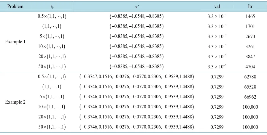
≤ or kmax=100000. In the table of the test results, t0 denotes initial point,
*
x denotes the solution, val denotes the final value of
( )
1( )
22
t H t
θ = , Itr denotes the number of iteration.
Example 1. Considering SGLCP with
( )
1
3
1 0
2 3
1 1
2 3
0 1
2
M
ω
ω ω
ω
+ −
= − + −
− +
, 1
( )
1 2 1 2 1 2
q
ω
ω ω
ω +
= +
+
,
( )
2
5
1 0
2 5
1 1
2 5
0 1
2
M
ω
ω ω
ω
+ −
= − + −
− +
, 2
( )
11
1
q
ω
ω ω
ω
+
= +
+
,
{
} { }
1 ω ω1, 2 0,1
Table 1. Results of the numerical Example 1-2 using method 1.
Problem t0 x∗ val Itr
Example 1
(
)
0.5×1,1,,1
(
−0.8385, 1.0548, 0.8385− −)
3.3 × 10⁻³ 1465(
1,1,,1)
(
−0.8385, 1.0548, 0.8385− −)
3.3 × 10⁻³ 1701(
)
5×1,1,,1
(
−0.8385, 1.0548, 0.8385− −)
3.3 × 10⁻³ 2670(
)
10×1,1,,1
(
−0.8385, 1.0548, 0.8385− −)
3.3 × 10⁻³ 3261(
)
20×1,1,,1
(
−0.8385, 1.0548, 0.8385− −)
3.3 × 10⁻³ 3847(
)
50×1,1,,1
(
−0.8385, 1.0548, 0.8385− −)
3.3 × 10⁻³ 4704Example 2
(
)
0.5×1,1,,1
(
−0.3747,0.1516, 0.0276, 0.0770,0.2306, 0.9539,1.4488− − −)
0.7299 62788(
1,1,,1)
(
−0.3746,0.1516, 0.0276, 0.0770,0.2306, 0.9539,1.4488− − −)
0.7299 65528(
)
5×1,1,,1
(
−0.3746,0.1516, 0.0276, 0.0770,0.2306, 0.9539,1.4488− − −)
0.7299 66962(
)
10×1,1,,1
(
−0.3746,0.1516, 0.0276, 0.0770,0.2306, 0.9539,1.4488− − −)
0.7299 100,000(
)
20×1,1,,1
(
−0.3746,0.1516, 0.0276, 0.0770,0.2306, 0.9539,1.4488− − −)
0.7299 100,000(
)
50×1,1,,1
(
−0.3746,0.1516, 0.0276, 0.0770,0.2306, 0.9539,1.4488− − −)
0.7299 100,000Example 2. Considering SGLCP with
( )
1
1
2 2 2 2 2 2
2 1
0 2 2 2 2 2
2 1
0 0 2 2 2 2
2 1
0 0 0 2 2 2
2 1
0 0 0 0 2 2
2 1
0 0 0 0 0 2
2 1
0 0 0 0 0 0
2 M ω ω ω ω ω ω ω ω + + + = + + + +
, 1
( )
3 2 3 2 3 2 3 2 3 2 3 2 3 2 q ω ω ω ω ω ω ω ω − + − + − + = − + − + − + − + ,
( )
1 32 2 2 2 2 2
2 3
0 2 2 2 2 2
2 3
0 0 2 2 2 2
2 3
0 0 0 2 2 2
2 3
0 0 0 0 2 2
2 3
0 0 0 0 0 2
2 3
0 0 0 0 0 0
2 M ω ω ω ω ω ω ω ω + + + = + + + +
, 1
( )
{
} { }
1 ω ω1, 2 0,1
Ω = = and pi=P
(
ωi∈ Ω =1)
0.5, i=1, 2. The test results are listed in “Table 1” using different initial points.5. Conclusion
In this paper, we present a new conjugate gradient projection method for solving stochastic generalized linear complementarity problems. The global convergence of the method is analyzed and numerical results show that Method 1 is effective. In future work, large-scale stochastic generalized linear complementarity problems need to be studied and developed.
Acknowledgements
This work is supported by National Natural Science Foundation of China (No. 11101231, 11401331), Natural Science Foundation of Shandong (No. ZR2015AQ013) and Key Issues of Statistical Research of Shandong Province (KT15173).
References
[1] Chen, X. and Fukushima, M. (2005) Expected Residual Minimization Method for Stochastic Linear Complementarity Problems. Mathematics of Operations Research, 30, 1022-1038.
http://www-optima.amp.i.kyoto-u.ac.jp/~fuku/papers/SLCP-MOR-rev.pdf
http://dx.doi.org/10.1287/moor.1050.0160
[2] Chen, X., Zhang, C. and Fukushima, M. (2009) Robust Solution of Monotone Stochastic Linear Complementarity Problems. Mathematical Programming, 117, 51-80. http://link.springer.com/article/10.1007/s10107-007-0163-z
http://dx.doi.org/10.1007/s10107-007-0163-z
[3] Lin, G.H. and Fukushima, M. (2006) New Reformulations for Stochastic Nonlinear Complementarity Problems. Opti-mization Methods and Software, 21, 551-564.
http://web.a.ebscohost.com/ehost/detail/detail?sid=beded7da-701c-4790-b1c9-81d20182cd04%40sessionmgr4005&vid =0&hid=4201&bdata=Jmxhbmc9emgtY24mc2l0ZT1laG9zdC1saXZl&preview=false#AN=22089195&db=aph
http://dx.doi.org/10.1080/10556780600627610
[4] Lin, G.H., Chen, X. and Fukushima, M. (2010) New Restricted NCP Functions and Their Applications to Stochastic NCP and Stochastic MPEC. Optimization, 56, 641-653.
http://www.amp.i.kyoto-u.ac.jp/tecrep/ps_file/2006/2006-011.pdf
http://dx.doi.org/10.1080/02331930701617320
[5] Ling, C., Qi, L., Zhou, G. and Caccetta, L. (2008) The SC 1 Property of an Expected Residual Function Arising from Stochastic Complementarity Problems. Operations Research Letters, 36, 456-460.
http://espace.library.curtin.edu.au/cgi-bin/espace.pdf?file=/2009/07/20/file_27/119233
http://dx.doi.org/10.1016/j.orl.2008.01.010
[6] Fang, H.T., Chen, X.J. and Fukushima, M. (2007) Stochastic ℜ0 Matrix Linear Complementarity Problems. SIAM
Journal on Optimization, 18, 482-506. http://www.polyu.edu.hk/ama/staff/xjchen/SIOPT_FCF.pdf
http://dx.doi.org/10.1137/050630805
[7] Gürkan, G., Ozge, A.Y. and Robinson, S.M. (1999) Sample-Path Solution of Stochastic Variational Inequalities. Ma-thematical Programming, 84, 313-333. http://link.springer.com/article/10.1007/s101070050024
http://dx.doi.org/10.1007/s101070050024
[8] Sun, Q.Y., Wang, C.Y. and Shi, Z.J. (2006) Global Convergence of a Modified Gradient Projection Method for Con-vex Constrained Problems. Acta Mathematicale Applicatae Sinica, 22, 227-242.
http://link.springer.com/article/10.1007/s10255-006-0299-2
http://dx.doi.org/10.1007/s10255-006-0299-2
[9] Wang, C.Y. and Qu, B. (2002) Convergence of the Gradient Projection Method with a New Stepsize Rule. Operations Research Transactions, 6, 36-44.
http://www.cnki.net/KCMS/detail/detail.aspx?QueryID=0&CurRec=4&recid=&filename=YCXX200201004&dbname =CJFD2002&dbcode=CJFQ&pr=&urlid=&yx=&v=MDM0OTdJUjhlWDFMdXhZUzdEaDFUM3FUcldNMUZyQ1V STHlmWXVadUZ5N2xWcnpJUEM3VGRyRzRIdFBNcm85Rlk
http://d.g.wanfangdata.com.cn/Periodical_yysxxb201004008.aspx
[11] Jing, S.J. and Zhao, H.Y. (2014) Conjugate Gradient Projection Method of Constrained Optimization Problems with Wolfe Stepsize Rule. Journal of Mathematics, 34, 1193-1199.