Effects of World Price and Oil Export Price Increases in the Framework of One sector and Two Sector Stylized Models

Munich Personal RePEc Archive

Effects of World Price and Oil Export

Price Increases in the Framework of

One-sector and Two-Sector Stylized

Models

Kapsalyamova, Zhanna

Christian Albrechts University of Kiel

10 November 2009

Online at

https://mpra.ub.uni-muenchen.de/18800/

Effects of World Price and Oil Export Price Increases in the Framework of One-sector and Two-Sector Stylized Models1

Working paper

Zhanna Kapsalyamova2

Christian Albrechts University of Kiel

Abstract

Interesting stylized models that discuss the implications of the oil boom or oil export price increase on an oil-rich economy must involve a tension between effects that tend to boost oil sector and harm non-oil sector and effects that vice versa tend to boost non-oil sector and harm oil sector. This paper explores such models and examines at large the implications of the oil export price increase through the prism of interaction between these two effects. This paper applies the 1-2-3-model of Devarajan et al. (1990) and develops two stylized models that examine the effects of the world price increase and oil export price increase on the economy respectively. A central feature of the developed stylized models is that they can distinguish between the two effects generated by the oil export price increase, namely the balance-of-trade effect and the import-competing effect. The balance-of-trade effect shows the response of the economy to the oil export price increase, depending on whether the economy runs a trade surplus or a trade deficit in the benchmark equilibrium, with the import-competing effect set equal to one. It shows conditions that cause changes in the producers’ real costs and hence determines which sector grows and which sector shrinks in the wake of the oil export price increase. The import-competing effect, under the assumption that trade is balanced, shows the effect of the variation in the Armington elasticity of substitution between oil goods in the second model and non-oil goods in the third model. It shows how competition between imported and import-competing goods affects producers’ real costs and hence determines which sector grows and which sector shrinks in the wake of the oil export price increase.

1. Introduction

In this paper, I apply the 1-2-3 model of Devarajan et al. (1990) and develop two stylized models to trace the effects of the increase in the world price of exported commodity in general and the increase in the oil export price in particular. I use the 1-2-3 model of Devarajan et al. (1990) because it represents a consistent framework for the analysis of general type of shocks such as world price increase, which is useful to examine before the effects of a particular type of shock such as an oil export price increase are considered.

I develop two stylized models that examine the effects of the oil export price increase because the literature in this area suffers from certain shortcomings. Firstly, it uses the Salter-Swan

1

I am grateful to Prof. Broecker and Prof. Rehdanz from Christian Albrechts University of Kiel for their invaluable comments on the earlier drafts of this paper.

2

framework, which does not incorporate two-way trade via assuming pure traded or nontraded sectors (e.g., Corden and Neary, 1982, Corden, 1984, Neary and van Wijnbergen, 1986). Incorporation of two-way trade in the model is important given that the extent of tradability of some good might be an important factor that determines the extent of the influence of an oil

export price increase on the sector producing this good. Or secondly, even if it incorporates

two-way trade, it considers the oil sector an enclave, and thus circumvents considering factor movement across the oil and non-oil sectors (e.g., Benjamin et al., 1989). Thus, to overcome the shortcomings in the literature, it is necessary to reassess the existing models via incorporating

two-way trade3 and factor movement into the model.

For these purposes, I develop two stylized models that assume two sectors: the oil sector, on the one hand, and the non-oil sector, on the other hand, that employ two factors in production: labor and capital. To introduce factor movement, I assume that labor is perfectly mobile, while capital is sector specific. The main difference between the two models is that they incorporate two-way trade in commodities differently. One of the models considers three types of oil commodities, exported oil, domestically sold oil, and imported oil, and one non-oil commodity, which is treated as nontraded. It is necessary to note that exported and domestically sold oil commodities are transformable into each other, whereas domestically sold4 and imported oil commodities are substitutable for each other. The other model assumes two oil commodities, exported oil and domestically sold oil, and two oil commodities, domestically sold oil and imported non-oil. Note that here two types of oil commodities are transformable into each other and two types of non-oil goods are substitutable for each other.

It is necessary to note that there are a number of possible combinations of assumptions about the transformability and substitution between goods that might be considered and I have chosen to concentrate on the two that appear to be the most appealing.5 To summarize again, the second model assumes transformability and substitutability between oil goods only, and the third model assumes transformability between oil goods and substitutability between non-oil goods. I perform this analysis to identify how the assumption of two-way trade might affect the results.

A central feature of the two-model analysis is that it can distinguish between the two effects generated by the oil export price increase, namely the balance-of-trade effect and the import-competing effect. The balance-of-trade effect shows the response of the economy to the oil export price increase, depending on whether the economy runs a trade surplus or a trade deficit in the benchmark equilibrium, with the import-competing effect set equal to one. It shows conditions

that cause changes in the producers’ real costs. The import-competing effect, under the

assumption that trade is balanced, shows the effect of the variation in the Armington elasticity of substitution between oil goods in the second model and non-oil goods in the third model. It

3

Note that two way trade in the model is conventionally introduced using Armington approach that assumes that there is substitutability (transformability) between imported and domestic goods (between exported and domestically sold goods).

4

It is necessary to note that the assumption of substitutability between domestically sold oil and imported oil already incorporates equilibrium condition at the markets for domestically supplied and demanded oil that implies that in the equilibrium the quantity of domestically sold oil and the quantity of domestically supplied and demanded oil are equal.

5

shows how competition between imported and import-competing goods affects producers’ real costs.

In general, the models considered in this paper share two common features. First, they do not

take into account monetary features; only relative prices are determined. Second, they are purely

neoclassical, so that there are no distortions in the commodities and factor markets. Eventually, everything returns back to the equilibrium after the benchmark equilibrium is distorted.

It is necessary to note that the analysis can equally be applied to cases in which the booming sector is not of an extractive type. It can be any other sector that enjoys positive terms of trade in the world markets. This is because I am concerned with the medium-run effects of the boom in the oil sector on resource allocation and income distribution, rather than with long-run issues such as the depletion of oil resources.

Overall, the paper consists of five sections. Section 2 discusses the effects of a world price increase using the 1-2-3 model of Devarajan et al. (1990). Section 3 describes the effects of an oil export price increase using a model that assumes differentiation of oil across its domestic sales, exports, and imports, and treats non-oil goods as nontraded. Section 4 covers an alternative variation of the model that assumes differentiation of oil across its domestic and foreign sales and differentiation of non-oil across imports and domestic sales. Section 5 concludes.

2 One-Sector Model

2.1 Overview of the Model

This section discusses the effects of the increase in the world price of exported commodity in the framework of the 1-2-3 model of Devarajan et al. (1990). The 1-2-3 model of Devarajan et al. (1990) is a standard one-country, two-sector, and three-commodity model. Essentially, the model considers only one aggregate sector that produces two commodities, exported and domestically supplied commodities, which the model treats as two different sectors. Given that the models to follow incorporate two sectors, namely the oil and non-oil sectors, I label this model a one-sector model for the sake of consistency.

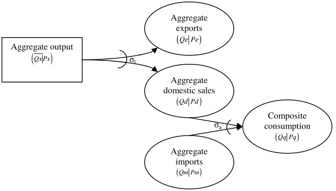
The model assumes aggregate output produced in the economy, or GDP, is fixed. Two-way trade is incorporated via assuming differentiation between domestic and foreign sales and between imports and domestically produced and domestically consumed goods (or import-competing goods). Thus, aggregate output is transformable into exports and domestic sales, combined via a

CET 6 function with an elasticity of transformation σ_{t. Imported and domestically sold}

commodities are imperfect substitutes. They are jointly combined via the CES7 function, which

includes the Armington elasticity of substitution σ_{a (see Figure 1). The mathematical notation}

used in the model is explained in Appendix A.1. The formulation of the model is presented in Appendix A.2.

2.2 Graphical Analysis of the Model

I show the effects of the world price increase by means of a graphical tool developed by Devarajan et al. (1990) (see Figure 2). Analogously to their diagram, the first quadrant depicts balance of trade, which is assumed to be balanced here. The second quadrant depicts a “consumption possibilities frontier” that shows a set of imports and domestic goods a household can buy at the corresponding prices. The third quadrant depicts the equilibrium in the domestic market. And the fourth quadrant depicts the production possibilities frontier or transformation curve across exports and the domestic supply given the corresponding prices. The diagram is drawn under the assumption that all prices are initially set equal to one. The points in the diagram, T and X, show the benchmark allocations of exports and the supply of the domestic commodity in the domestic markets, and imports and the demand for domestic commodities, respectively.

6

CET stands for constant elasticity of transformation. 7

CES stands for constant elasticity of substitution.

Aggregate output

(

Qx Px

)

Aggregate exports

(Qe Pe)

Aggregate domestic sales

(Qd Pd)

Aggregate imports

(Qm Pm)

Composite consumption

(Qq Pq)

σ_t

[image:5.612.114.453.105.298.2]

σ_a

Figure 1 Flows of commodities in a one-sector model

I assume that the world price of the exported commodity rises, or in other words, the terms of trade improve. This shifts the trade balance line counterclockwise. Now, for a given export, the household can buy more imports. This is achieved via real exchange rate appreciation. Note that imports increase unambiguously and the real exchange rate always appreciates except for the case when imports and domestically supplied commodities are perfect substitutes, when no change in the real exchange rate occurs.

The real exchange rate appreciation leads to further adjustments in exports and domestic supply. Whether there is an increase in exports or domestic supply depends on the extent of the import-competing effect, defined as a variation in the Armington elasticity of substitution. If domestic commodities and imports are gross substitutes

(

σ

_a >1

)

, or the import-competing effect is high, as shown in the diagram, exports rise and supply of domestic goods falls. In the opposite case, when goods are gross complements

(

σ

_a <1

)

, or the import-competing effect is low, the supply of

domestic good rises and exports fall. They remain unchanged if

σ

_a =1.

In light of the growing demand and adjustments in relative prices, the household tends to prefer imported goods to domestically supplied goods if they are gross substitutes, and does not have

Qe Qm

d

Qd

s

Qd

I II

III IV

T * T X

* X

( , d)

Qq= f Qm Qd Trade balance

Domestic market

( , )

[image:6.612.100.470.367.676.2]

Qx= f Qe Qd

strong preferences over any of them if they are gross complements. In the former case, as a result of the strong competition, domestic sales decrease and in the latter they increase. Given that exports and domestic sales are transformable and aggregate output is exogenous, an increase in one of them should necessarily decrease the other. Therefore, exports and domestic supply move in opposite directions in the wake of the world price increase.

The results of the model can be shortly summarized as follows. First, the real exchange rate always appreciates, except for the case when

σ

_a → ∞, when it remains unchanged. Second, imports unambiguously increase, whereas domestic sales and exports are ambiguous and tend to move in opposite directions.

The model that I considered here is very general. Even though the results are fundamental, the model fails to capture intersectoral allocation, which would prove useful when studying the effects of the particular type of shock. Given that oil export price increase effects are a particular subject of this study, I extend the present model to two-sector model in what follows.

3. Stylized two-sector model

In this section, I develop a stylized two-sector model with two factors used in production. In what follows, I give an overview of the key features of the model and proceed with an analysis of the core effects responsible for structural adjustments.

3.1 Overview of the Model

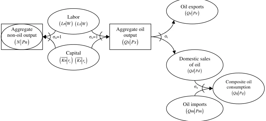
This is a model of a two-sector economy, with two sectors producing oil and non-oil goods. I assume that the oil sector is a traded sector and the non-oil sector is a purely nontraded sector. The domestic economy exports oil, supplies oil domestically, and imports oil, but consumes all of the non-oil produced domestically.

It is necessary to note that the two-way trade is incorporated into the model via assuming differentiation between domestic and foreign sales of oil and between imports and domestically consumed oil (or import-competing oil). Aggregate oil is transformable into exports and domestic sales of oil. Imports and domestically consumed oil are imperfect substitutes.

I assume two production factors: labor and capital. To reflect the medium-term, I assume capital is sector-specific and labor is mobile across sectors. The model is purely neoclassical, with no rigidities assumed. The wage rate clears the labor market, with full employment achieved in the equilibrium. The model abstracts from intermediate goods, taxes, and transaction costs. It treats trade balance as exogenous and exchange rate as endogenous. The complete formulation of the model and its solution is given in Appendix B.2.

3.2 Analysis of the Model: Disaggregation of Effects

By and large, there are two key effects that explain the response of the economy in the model. The first effect is labeled a balance-of-trade effect and the second an import-competing effect. I examine the two effects in isolation.

The balance-of-trade effect shows the response of the economy to the oil export price increase, depending on whether the economy runs a trade surplus or trade deficit in the benchmark

Aggregate oil output

(

Qx Px

)

Oil exports (Qe Pe)

Domestic sales of oil

(Qd Pd)

Oil imports

(Qm Pm)

Composite oil consumption

(Qq Pq)

σ_t

σ_a

Labor

(Ln W) (Lx W)

Capital

(

Kn rx

)

(

Kx rn

)

Aggregate

non-oil output

(

N Pn

)

σo=1

[image:8.612.69.533.128.340.2]

σn=1

Figure 3 Production technology and flows of the commodities in the stylized two-sector model

equilibrium, with the import-competing effect set equal to one.8 It shows the conditions that cause changes in the producers’ real costs. The import-competing effect, under assumption that trade is balanced, shows the effect of the variation in the Armington elasticity of substitution between oil goods. It shows how competition between imported and import-competing oil goods affects producers’ real costs. It is necessary to note that as I assume substitution between oil goods, the import-competing effect is associated with the variation in the Armington elasticity of substitution between oil goods. In the subsections 3.2.1 and 3.2.2, the impact of each of the two effects is considered in isolation. The results under each particular effect are summarized in Table 1.

3.2.1 Balance-of-Trade Effect

The balance-of-trade effect encompasses the roleof a trade deficit or surplus on the economy. To provide a clearer understanding of the effect, I present an intuitive analysis here.

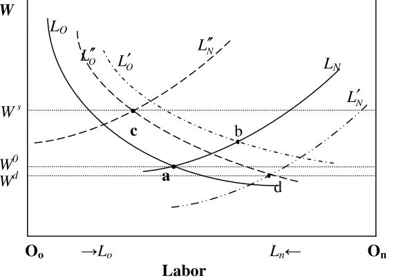
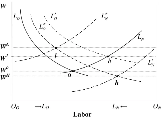
I begin the analysis by examining the labor market. Using Figure 4,9 I illustrate the behavior of the labor market in the benchmark equilibrium and after the oil export price increases. On the horizontal axis, I depict the total labor supply and on the vertical axis the wage rate in terms of the aggregate price of oil. The amount of labor employed in the oil sector is measured starting from Oo and in the non-oil sector starting from On. Given that the model assumes the labor supply

is exogenous, full employment should always be maintained in the equilibrium. The labor demand schedules (LO and LN) are drawn with negative slopes, implying that they are decreasing

functions of the wage rate.^

An increase in the oil export price leads to an increase in the unit revenue of the oil producer (Px) or in other words to an increase in theaggregate oil price. This trend in its turn causes an increase in the demand for labor in the oil sector, illustrated in Figure 4 by the shift of the labor demand schedule to the right, from L_Oto L_O′ , since, for a given wage rate, the oil producer’s marginal revenue product rises. The economy reaches point b, at which the real wage increases and labor moves from the nontraded sector into the oil sector. However, note that this is not a final outcome.

Given that the economy pursues the same pattern of foreign trade as in the benchmark scenario, and this pattern is implied by the exogenous balance of trade, an increase in exports should be accompanied by an increase in imports. This is achieved via appreciation of the real exchange rate. This appreciation in its turn reduces the unit revenue of the oil producer. This trend is illustrated in Figure 4 by the shift of the labor demand schedule leftwards from L_O′ to L_O′′. To determine how demand for labor from the non-oil sector changes, I first have to define the change in total income after the oil export price increases.

8

This is in line with the results delivered by the previous one-sector model. It was found that as long as the import-competing effect is equal to unity, there are no changes in most of the quantities.

9

Note: The initial benchmark labor supply and demand schedules before an oil export price increase are shown using solid lines, whereas after an oil export price increase they are shown using dashed lines.

It is necessary to note that the total income accruing to the economy (Y), or in other words GNP, depends strongly on the pattern of foreign trade. If the pattern of trade remains the same, it is essential to distinguish between the cases when the economy has a trade surplus and when it has a trade deficit. If the economy accumulates a trade surplus, GNP increases, otherwise if the economy runs a trade deficit, GNP decreases. Naturally, a trade surplus generates additional revenue for the economy, as a result of which GNP increases, whereas with a trade deficit the opposite occurs. Thus, GNP depends strongly on the pattern of trade in the benchmark.

I consider first the case when the economy accumulates a trade surplus in the benchmark. If the economy enjoys a trade surplus, its income rises as a result of the oil export price increase. This trend leads to an increase in the demand for goods sold domestically, in particular for nontraded non-oil goods. This increase in demand causes the non-oil price to increase relative to the aggregate oil price. The increase in the relative non-oil price decreases the real costs of labor of the non-oil producer relative to the oil producer, and hence leads to an increase in the employment in the non-oil sector. This effect is illustrated in Figure 4 by the shift of the labor demand schedule for the non-oil producer to the left, from L_N to L_n′′. The new equilibrium is achieved at point c, which is associated with an increase in the real wage in terms of the oil producer’s aggregate price, a decrease in employment in the oil sector, and an increase in employment in the non-oil sector.

If the country runs a trade deficit, appreciation of the exchange rate will exert a downward pressure on income. This in turn reduces demand and the relative price for non-oil, which further

•

W

Oo →Lo Ln← On Labor

a

W0

b

• •

c

LO

LN

Wd

O

L′ N

L′′

N

L′

s

W

O

L′′

•

[image:10.612.105.390.144.347.2]

d

leads to a decline in employment in the non-oil sector and thus causes its further contraction. Graphically, the trade deficit case is depicted by the shift of the labor demand schedule in the non-oil sector rightwards to L_N′ . The new equilibrium is achieved at point d, which is associated with a drop in wage in terms of the aggregate oil price, an increase in employment in the oil sector, and a decrease in employment in the non-oil sector.

With activity-specific capital and an absence of intermediate goods, the change in employment largely defines the equilibrium response of the aggregate oil and non-oil outputs. At this juncture, it can be concluded that in the trade surplus case, the aggregate output of the oil sector falls and the output of the non-oil sector rises. In the trade deficit case the opposite occurs. The results are summarized in the Table 1, where up and down arrows indicate an increase and a decrease in the corresponding variable.

[image:11.612.64.517.309.602.2]

Table 1 The effects of the oil export price increase under alternative scenarios

Balance-of-trade effect Import-competing effect No Variable

Trade deficit

Trade surplus

1 <

a

σ

σ

_a >1

1. Qx ↑ ↓ =0 =0

2. N ↓ ↑ =0 =0

3. Qe ↑ ↓ ↓ ↑

4. Qm ↑ ↑ ↑ ↑

5. Qd ? ? ↑ ↓

6. Qq ? ? ↑ ↑

7. Pe ↑ ↓ ↓ ↑

8. Pd ↓ ↑ ↑ ↓

9. Pm ↓ ↓ ↓ ↓

10. Px10 - - - -

11. Pn ↓ ↑ =0 =0

12. Pq ↓ ? ↓ ↓

13. W ↓ ↑ =0 =0

14. Lx ↑ ↓ =0 =0

15. Ln ↓ ↑ =0 =0

16. R ↓ ↓ ↓ ↓

17. Y ↓ ↑ =0 =0

Note: Arrows pointing up (down) indicate an increase (decrease) in the corresponding variables. A question mark indicates that the effect on the variable is ambiguous. The notation used here is explained in Appendix B.1.

So far, I have largely discussed effects of the oil export price increase on the factor markets and aggregate commodities. In what follows, I turn the focus to adjustments in the quantities of disaggregated commodities.11 Quantities of disaggregated commodities primarily change due to

10

Px is treated as a numeraire. 11

expansion and substitution effects. The expansion effect arises due to the change in the aggregate quantities, such as Qx and Qq, whereas the substitution effect arises due to the change in the corresponding relative prices.

In the trade deficit case, the oil export price (Pe) rises and the domestic oil price (Pd) falls. Given that the aggregate output of oil (Qx) increases, oil exports rise unambiguously due to positive expansion and substitution effects. However, the change in the domestic consumption of oil (Qd) is ambiguous due to a positive expansion effect and a negative substitution effect. Oil imports rise unambiguously.

In the trade surplus case, exports of oil fall unambiguously, but the change in the domestic supply of oil is ambiguous due to negative expansion and positive substitution effects. The final change in the quantity of the domestic supply of oil depends on which of the effects dominates. Oil imports rise unambiguously.

3.2.2 Import-Competing Effect

The import-competing effect encompasses the effect of the Armington elasticity of substitution between oil goods on the economy.

With balanced trade, the model replicates the results of the one-sector model described earlier in Section 2.12 Thus, it can be concluded that import-competing effect alone under the assumption that trade is balanced does not engender factor movement across sectors and thus has no effect on the outputs of either the oil or non-oil sectors. The import-competing effect affects only disaggregated commodities, such as exported oil, domestically sold oil, and imports of oil, and their corresponding relative prices.

In the framework of the present model, given balanced trade, there is no change in total income, and no change in the demand pattern: what is earned additionally, for instance, from producing aggregate oil is spent on the consumption of composite oil and the consumption of non-oil. Consumption patterns do not change. By and large, increase in consumption does not cause the price of non-oil to change vis-à-vis the aggregate price of oil, and as a result there is no factor movement across sectors and hence no change in the outputs of oil and non-oil goods.

Given that I have provided a lengthy discussion of the results with respect to the disaggregated commodities in Section 2, I will not repeat this analysis here to save space.

4 Alternative Variation of the Stylized Two-Sector Model

4.1 Overview of the Model

12

The model discussed in this section is slightly different from the model in the previous section in that it treats commodities differently. In the previous model, I considered three types of oil goods and one type of non-oil good, which was treated as nontraded. In this section, I consider only two types of oil goods, an oil good that is exported (Qe) and an oil good that is supplied domestically (Qd), but two types of non-oil goods, a non-oil good that is produced domestically (N) and a non-oil good that is imported (Qm). Unlike the previous model, the current model assumes no imports of oil and no pure nontraded goods.

Similar to the previous model, oil and non-oil goods are produced using labor and capital. Capital is sector specific and labor is perfectly mobile across sectors. It is a neoclassical world; hence, the wage is used to clear labor market so that full employment is achieved. The formulation of the model is shown in Appendix C.2.

Figure 5 shows production technology and flows of commodities. The household owns all the sectors and thus receives all the income accruing to the economy. The rest of the world supplies non-oil (Qm) to the domestic economy and consumes exports of oil (Qe).

4.2 Analysis of the Model: Disaggregation of Effects

Similar to the previous model, there are two key effects that determine the response of the economy to the oil export price increase: the balance-of-trade effect and the import-competing

effect. It is necessary to note that given that the current model assumes substitutability between non-oil goods, whereas the previous model assumed substitutability between oil goods, the import-competing effect in the current model is different from the import-competing effect in the previous model. To evaluate the impact of the variation in the Armington elasticity of

Aggregate non-oil output

(

N Pn

)

Aggregate oil output

(

Qx Px

)

Oil exports (Qe Pe)

Domestic sales of oil

(Qd Pd)

Non-oil imports

(Qm Pm)

Composite non-oil consumption

(Qq Pq)

σ_t

σ_a

Labor

(Ln W) (Lx W)

Capital

(

Kn rx

)

(

Kx rn

)

σo=1

[image:13.612.72.534.358.509.2]

σn=1

Figure 5 Production technology and flows of commodities in the alternative variation of two-sector model

substitution between non-oil goods on the economy, I have to consider a different treatment of the non-oil goods in this model than I did in the previous model.

4.2.1 Balance-of-Trade Effect

The balance-of-trade effect determines how trade deficit or trade surplus affects the economy if the Armington elasticity of substitution between non-oil goods is set equal to one. The trade surplus effect favors non-oil production, whereas the trade deficit favors oil production. The same reasoning applies here as in the previous model. Given the constant pattern of trade in the world markets, in the case of a trade surplus, the real exchange rate appreciation increases total income. As a result, non-oil production grows and oil production shrinks. In the case of trade deficit, the opposite occurs, namely non-oil production shrinks and oil production expands. In general, the effects of the balance-of-trade effect under the two different models are similar. The key results are shown in the Table 2.

4.2.2 Import-Competing Effect

In this section, I discuss the effects of the import-competing effect when trade is balanced. Balanced trade implies that the following conditions should hold:

γ γ

ρ ϕ

− =

= − −

1 )

2

0 1

) 1

The first condition states that the share of the trade balance in total income is zero. The second condition states that, given that I assume one import and one export good, their shares in their balance of trade are equal.

[image:15.612.66.521.98.404.2]

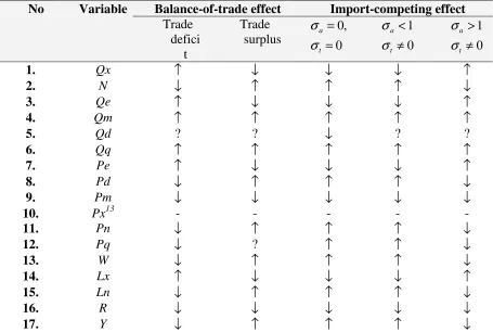
Table 2 The effects of the oil export price increase: results from the alternative model

Balance-of-trade effect Import-competing effect No Variable

Trade defici

t

Trade surplus

0 , 0 =

=

t a

σ σ

0 1 ≠

<

t a

σ σ

0 1 ≠

>

t a

σ σ

1. Qx ↑ ↓ ↓ ↓ ↑

2. N ↓ ↑ ↑ ↑ ↓

3. Qe ↑ ↓ ↓ ↓ ↑

4. Qm ↑ ↑ ↑ ↑ ↑

5. Qd ? ? ↓ ? ?

6. Qq ↑ ↑ ↑ ↑ ↑

7. Pe ↑ ↓ ↓ ↓ ↑

8. Pd ↓ ↑ ↑ ↑ ↓

9. Pm ↓ ↓ ↓ ↓ ↓

10. Px13 - - - - -

11. Pn ↓ ↑ ↑ ↑ ↓

12. Pq ↓ ? ↑ ↑ ↓

13. W ↓ ↑ ↑ ↑ ↓

14. Lx ↑ ↓ ↓ ↓ ↑

15. Ln ↓ ↑ ↑ ↑ ↓

16. R ↓ ↓ ↓ ↓ ↓

17. Y ↓ ↑ ↑ ↑ ↓

Note: Arrows pointing up (down) indicate increase (decrease) in variables. A question mark indicates that the effect on the variable is ambiguous. The notation used here is explained in Appendix C.1.

In what follows, I determine the response of the economy under low

(

σ_a <1

)

and high

(

σ_a >1

)

import-competing effects. The results are summarized in Table 2.

Low import-competing effect

In what follows, I consider a special case of the low import-competing effect

(

σ_a <1

)

, namely a case in which there is no import-competing effect

(

σ

_a =0

)

, or other words a case in which non-oil imports and domestically produced non-non-oil are pure complements. I consider this case because it is easier to understand and because it has tractability advantages. I should note that the results derived are valid for the low import-competing scenario overall.

The adjustments in the labor market are illustrated in Figure 6. Here, there are two round effects. In the first round after the oil export price increases, the unit revenue of the oil producer (Px) rises. This reduces the oil producer’s costs and increases her labor demand. Graphically, it is illustrated via the shift of the labor demand schedule to the right, from LO to LO′ . In the second

round, given that trade must be kept in balance, an increase in the value of oil exports engenders

13_Px

an increase in the quantity of non-oil imports. This is achieved via real appreciation of the exchange rate. This trend in its turn reduces the oil producer’s unit revenue and hence causes the labor demand schedule to shift back to the left, to L_O′′.

Becauseincome rises, the demand for commodities sold domestically rises, and because domestic non-oil and imported non-oil are complements, the aggregate price of non-oil (Pn) rises as well. This trend causes an increase in the demand for labor in the non-oil sector, illustrated by the shift of the non-oil sector’s labor demand schedule to the left, from LN toLN′′. Eventually, the real wage

in terms of the oil producer’s unit of revenue increases. Hence, the equilibrium employment in the non-oil sector increases and the equilibrium employment in the oil sector decreases. As a result, the non-oil sectorexpands and the oil sector contracts.

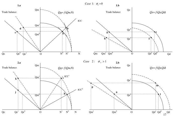
The impact of the oil export price increase on disaggregated commodities and prices is illustrated in Figure 7. The upper part of the Figure (Graphs 1.a and 1.b) demonstrates the effects of the oil export price increase under a low import-competing effect and lower part (Graphs 2.a and 2.b) demonstrates effects of the oil export price increase under a high import-competing effect. The hand side of Graphs 1.a and 2.a shows the consumption possibility frontiers and the hand side of Graphs 1.b and 2.b shows the production possibility frontiers. In addition, the right-hand side of Graphs 1.a and 2.a show income consumption curves (ICCs). Given that non-oil goods are assumed to be perfect complements in the upper part of the figure, the income consumption curve is drawn as a 45 degree ray through the origin (O). The lower part of Figure 7 assumes that the goods are imperfect substitutes, and hence the income consumption curve is

•

W

OO →LO LN ← ON

Labor a

W0

WL

b

• •

l

W1

O

L

O

L′′

O

L′ L_N′′

N

L

N

L′

WH •

[image:16.612.122.402.206.412.2]

h

Figure 6 Effects of the oil export price increase on the labor market: import-competing effect

drawn with a slope different from the forty-five degree line. The left-hand side of all the graphs depicts trade balance. The axes of the graphs show quantities of exported oil (Qe), imported non-oil (Qm), domestically supplied oil (Qd) and non-oil produced domestically (N). Given that trade is balanced, with export prices set equal to one, the trade balance is represented by a 45 degree line that goes through the origin. Further, given the amount of imports and exports and their relative prices, the quantities of domestic non-oil (N) and oil (Qd) can be seen in from the right-hand side of the graphs.

The oil export price increase in Graphs 1.a and 1.b is depicted by the shift of the trade balance line clockwise and counterclockwise, respectively, which implies that for a given amount of exports one can buy more imports. The shift in the trade balance automatically translates into an asymmetric shift of the consumption possibility frontier, with the maximum amount of non-oil demanded being unaffected. However, this shift is associated with the increase in the maximum amount of imports by the amount equal to the increase in the imports per unit of exports after the oil export price increases.

Earlier in this section, I observed that when non-oil goods are gross complements, the non-oil sector expands and the oil sector contracts. Taking this into account, the production possibility frontier in Graph 1.b shifts inwards. As a result, exports decrease unambiguously because of the contraction of aggregate output (negative expansion effect) and the real appreciation of the exchange rate (negative substitution effect). However, the effect of the oil export price increase on domestic sales of oil is ambiguous. Domestic sales of oil decline as a result of the negative expansion effect and increase as a result of the positive substitution effect. The dominating effect determines the ultimate change in the domestic sales of oil. Graph 1.b is drawn under the assumption that the negative expansion effect dominates and hence Qd declines. The new equilibrium is reached at point f.

Increase in imports is unambiguous due to the increase in income and the appreciation of the real exchange rate. Given that Qm and N are assumed to be complements, as depicted by the fixed income consumption curve, both of them tend to rise as a result of the oil export price increase, as shown by the point b in Graph 1.a.

High import-competing effect

The high import-competing effect

(

σ

_a >1

)

is illustrated in Figure 6 and lower part of Figure 7 (Graphs 2.a and 2.b). I begin by analyzing the adjustments in labor market first. The labor demand schedule for the oil producer shifts first rightwards and later leftwards, first as a result of the oil export price increase and later as a result of the real exchange rate appreciation. Total income declines and hence demand for non-oil declines. This trend drives relative Pn down. As a result, employment in the oil sector increases and in the non-oil sector it decreases. The oil sector expands and the non-oil sector contracts. In Figure 6, the equilibrium in the labor market is illustrated at point h, where two labor demand schedules (L_O′′ and L_N′ ) intersect with each other.

Qe Qe1 Qe0 Qe0 Qe1 Qm1 Qm0

N0 N1

Qe0 Qe1 O

0 :

1 _a=

Case

σ

Qm N Qe Qe Qd Qm Qm1 Qm0 O Qd1 Qd0

• • • • • • • • • Qm Qm1 Qm0

1 0 1 0 1 0 1 0

1 :

2 _a >

Case

σ

) , (QeQd f

Qx=

[image:18.792.51.751.105.575.2]

) , (QmN f Qq= Trade balance Trade balance Trade balance ) , (QeQd f Qx= a b d c e f g h h i j k l m n p ) , (QmN f Qq= • • • • • • • • 1.a 1.b 2.a 2.b

Figure 7 Effects of the oil export price increase on the adjustments in the goods markets under different import- competing effects

ICC

ICC0 ICC1

5 Conclusions

In this paper, I highlighted the importance of the assumption of two-way trade and factor movement across sectors using two own models. I find that variation in the Armington elasticity of substitution between oil goods does not play a role for sectoral allocations, whereas variation in the Armington elasticity of substitution between non-oil goods plays a role.

In general, the two models pointed towards two effects triggered by the oil export price increase: a balance-of-trade effect and an import-competing effect. Unlike the predictions of the core Dutch disease model (e.g., Corden and Neary, 1982), I find that it is possible to expect that the non-oil sector expands and the oil sector contracts in the wake of an oil boom. In particular, in one stylized model, the balance-of-trade effect might either increase or decrease the outputs of the oil and non-oil sectors, whereas in the other stylized model both the balance-of-trade effect and import-competing effects might either increase or decrease the outputs of the oil and non-oil sectors.

In general, I find that the models deliver quite intuitive and plausible results. However, it is necessary to note that reality is more complex and incorporates other effects not captured by these models. In reality, there are more than two sectors; there is a room for savings and investment, etc. How would incorporating these features affect the results predicted by these models? These are the questions that I leave for the future research.

References

Benjamin, N. C., Devarajan, S. and Weiner R. J. (1989). The ‘Dutch’ disease in a developing country. Oil reserves in Cameroon. Journal of Development Economics, 30, 71-92. North Holland.

Corden W. (1984). Booming sector and Dutch Disease economics: survey and consolidation.

Oxford Economic Papers, 36, 359-380.

Corden W. and Neary, J. (1982). Booming sector and de-industrialisation in a small open economy. Economic Journal, 92, December, 825-848.

Devarajan, S., Lewis, J. D., and Robinson, S. (1990). Policy lessons from trade-focused, two-sector models. Journal of Policy Modelling, 12, 625-657.

Appendix A Description of the One-Sector Model

Appendix A.1 List of the Symbols Used in the One-Sector Model

Symbol Definition

PARAMETERS

α

Value share of domestic sales in the total production Px Qx

Qd Pd

× × =

α

1-

α

Value share of exports in the total production Px Qx

Qe Pe

× × = −α

1

t

σ Elasticity of transformation between exported and domestically supplied _commodities

a

σ Armington elasticity of substitution between imports and domestically _{consumed commodities}

β Value share of demand for import-competing commodity in the _{composite consumption} Pq Qq

Qd Pd

× × =

β

β

−

1 _{Value share of imports in composite consumption (or total absorption)} Pq Qq

Qm Pm

× × = −β

1

EXOGENOUS VARIABLES

pwm Import price in foreign currency units

z Export price in foreign currency units

Qx Quantity of total production or aggregate commodity

Pq Price of composite commodity Qq

ENDOGENOUS VARIABLES (explicitly shown in the model)

Outputs

Qm Quantity of imports

Qd

Quantity of domestically supplied and domestically demanded commodity or quantity of import-competing commodity

Qe Quantity of exports

Prices

Pm Import price in domestic currency units

Pd Price of domestically produced and domestically supplied commodity

Pe Export price in domestic currency

R Nominal exchange rate

ENDOGENOUS VARIABLES

(implied by the model but not explicitly shown in it)

Qq Quantity of composite consumption or total absorption

Appendix A.2 Overview of the One-Sector Model

In addition to the nonlinear representation of the model, I derive a log-linearized version of the model. In what follows, I place the percentage change form equations to the right of the nonlinear equations. A circumflex (^) denotes percentage change in the corresponding variable.

Given that the model ignores factor markets, aggregate output level, Qx, is exogenously given, and is defined as

(A.1.a)

(

(

)

)

1

1

t t t

t t

Qx= ×n δ ×Qdρ + −δ ×Qeρ ρ , (A.1.b) α×Qd+ −

(

1 α

)

×Qe=0,

where n is a CET function shift parameter, δ_t is a CET function share parameter, ρ_tis a CET function exponent and

α

is the value share of domestic sales in the aggregate output. Qd is the quantity of the commodity produced and supplied domestically (in what follows, I refer to it as a domestic commodity or import-competing commodity) andQe is the quantity of the commodity exported.

I assume that Qdand Qe are transformable, and the producer optimizes her production as follows:

(A.2.a)

t

c c

Pe Qe

Qd Pd

σ

λ

 

= × 

  , (A.2.b) Qe Qd− =

σ

t×

(

Pe−Pd

)

,

where Pe

(

defined below and

)

Pd are the prices of the exported good in domestic currency and

of domestic good, respectively, λ is a constant, and

σ

_t is the elasticity of transformation.

(A.3.a) Pe= ×z R, (A.3.b)Pe= +zˆ Rˆ,

where R is the exchange rate and z is a world price of the exported commodity.

The optimal allocation across the consumption of domestic and imported commodities is given as

(A.4.a)

a

Qm Pd

Qd Pm

σ

υ  

= ×_{ }

  (A.4.b) Qm Qd− =

σ

a×

(

Pd−Pm

)

,

(A.5.a) Pm= pwm R× , (A.5.b) Pm=Rˆ,

where pwm is the world price of the import.

I assume that foreign trade is balanced:

(A.6.a) pwm Qm× = ×z Qe, (A.6.b) Qm= +zˆ Qe,

I use the price of a composite commodity, Pq, as a numeraire:

(A.7.a) Pq= ×β Pd+ −

(

1 β

)

×Pm, (A.7.b) β×Pd+ −

(

1 β

)

×Pm=0,

with β being the share of consumption of the domestic commodity in total absorption.

By and large, the one-sector model is represented by seven equations with seven unknowns, i.e., ,

Appendix B Description of the Stylized Two-Sector Model

Appendix B.1 List of the Symbols Used in the Two-Sector Model

Symbol Definition

PARAMETERS

Greek letters

α Value share of domestic sales of oil in the output of aggregate oil Px Qx

Qd Pd × × = α

1-α Value share of exports of oil in the output of aggregate oil Px Qx

Qe Pe × × = −α 1 t

σ Elasticity of transformation between exported and domestically _{supplied oil}

a

σ Armington elasticity of substitution between imported and import-_{competing oil}

π Value share of labor employed in the aggregate oil output Px Qx

Lx w × × = π

1-π Value share of capital employed in the aggregate oil output Px Qx

Kx r × × = −π 1

ω Value share of labor employed in the aggregate non-oil output Pn N Ln w × × = ω

1-ω Value share of capital employed in the aggregate non-oil output Pn N Kn r × × = −ω 1

λ Share of labor employed in the oil sector L

Lx

=

λ

1-λ Share of labor employed in the non-oil sector L

Ln

= −λ 1

q

ψ _{Marginal propensity of consumption of composite oil} q Pq_YQq

× =

ψ

n

ψ _{Marginal propensity of consumption of composite non-oil} n Pn_Y N

× =

ψ

ϕ Value share of aggregate oil output in total income Y

Qx Px×

=

ϕ

ρ _{Value share of aggregate non-oil output in total income} ρ = Pn_Y×N

1-ϕ-ρ _{Share of the balance of trade in total income Y}

Bal R×

= − −ϕ ρ 1

γ _{Value share of oil imports in trade balance} Bal

Qm pwm×

=

γ

1-γ _{Value share of oil exports in trade balance Bal}

Qe z× = −γ 1 t

δ _{CET function share parameter}

t

θ Constant

χ _{Shift parameter in CES function}

q

δ _{CES function share parameter}

q

ρ _{CES function exponent}

υ Constant in the equation that determines optimal ratio of consumption of import-competing oil to imports of oil

Latin letters

a

Value share of oil imports in composite consumption of oil (or total

absorption of oil) Pq Qq

Qm Pm a

× × =

1-a

Value share of demand for import-competing oil in the composite

consumption of oil Pq Qq

Qd Pd a

× × = −

1

k Constant in the aggregate oil production function m Constant in the aggregate non-oil production function n CET function shift parameter

EXOGENOUS VARIABLES

pwm Import price of oil in foreign currency units z Export price of oil in foreign currency units

Bal Balance of trade or foreign savings

Px Price of aggregate oil, or unit revenue of oil producer (Numeraire)

L Total supply of labor

ENDOGENOUS VARIABLES (explicitly shown in the model) Factors

Lx

Quantity of labor employed in the oil sector

Ln

Quantity of labor employed in the non-oil sector

Outputs

Qx Quantity of aggregate oil N Quantity of aggregate non-oil Qm Quantity of oil imported

Qd Quantity of domestically supplied oil or quantity of import-competing oil Qe Quantity of exports of oil

Qq Quantity of composite oil or oil absorption

Prices

w Economywide wage rate

Pn Price of non-oil, or unit revenue of non-oil producer Pd Price of oil sold domestically

Pe Price of exported oil in local currency units Pm Import price of oil in domestic currency units

R Nominal exchange rate Pq Price of composite oil

MACRO VARIABLES

Y Total income

walras Artificial variable used to ensure that the number of unknowns is equal to the number of equations

(implied by the model but not explicitly shown in it)

rx Oil sector specific price of capital

rn Non-oil sector specific price of capital

Appendix B.2 Overview of the Stylized Two-Sector Model

In addition to the nonlinear representation of the model, I derive a log-linearized version of the model. In what follows, I place percentage form equations to the right of the nonlinear equations. As before, a circumflex (^) denotes percentage change in the corresponding variable:

(B.1.a) Qx=k×Lxπ, (B.1.b) Qx= ×π Lx,

(B.2.a) N =m×Lnω, (B.2.b) ˆN = ×ω Ln,

where Qx and N stand for quantities of aggregate oil and non-oil. Lx and Ln are quantities of labor employed in the oil and non-oil sectors, respectively. π and ω represent the value shares of the labor inputs in the outputs of aggregate oil and non-oil, respectively. k and m are constants.

The first-order conditions for employment of labor are

(B.3.a)

Lx Qx Px

w=π× × , (B.3.b) ˆw=Px Qx+ −Lx,

(B.4.a)

Ln N Pn

w=ω× × , (B.4.b) ˆw=Pn Qn+ −Ln,

where Px is the price of aggregate oil and Pn is the price of non-oil.

I differentiate oil commodities by their source of origin and destination, as in the previous section. The model accommodates two-way trade, by assuming qualitative differences between exported, imported, and domestically supplied oil. The output of aggregate oil is transformed into exports (Qe) and domestic sales (Qd) of oil via the CET function as follows:

(B.5.a) _{Qx n}

(

_Qd t

(

)

_Qe t

)

t

t t

ρ ρ

ρ _δ

δ × + 1− × 1

×

= , (B.5.b) Qx= ×α Qd+ −

(

1 α

)

×Qe,

where n is a CET function shift parameter, δ_t is a CET function share parameter, ρ_tis a CET function exponent, and α is the value share of domestic sales of oil in the output of aggregate oil.

The optimal allocation of aggregate oil across the quantities of exported (Qe) and domestically supplied oil (Qd) (or import-competing oil) is given by

(B.6.a)

t

Pd Pe Qd

Qe σ

θ 

     ×

= , (B.6.b) Qe Qd− =σ_t×

(

Pe−Pd

)

,

where Pe is the price of exported oil measured in local currency, Pd is the price of oil sold in the domestic market, θ is a constant, and σ_t is the elasticity of transformation between exports of oil and domestically supplied oil.

(B.7.a)

(

q

(

)

q

)

q

Qm Qd

Qq χ δ_q ρ δ_q ρ ρ

1

1 − −

−

× − + ×

×

= , (B.7.b) Qq= ×a Qm+ −

(

1 a

)

×Qd,

where Qm is the quantity of oil imported, χ is a shift parameter in the CES function, δ_q is a CES function share parameter, ρ_q is a CES function exponent, and a is the value share of oil imports in consumption of composite oil.

The optimal ratio of consumption of import-competing oil (Qd) to imports of oil (Qm) is

(B.8.a)

a

Pm Pd Qd

Qm σ

υ 

     ×

= , (B.8.b)Qm Qd− =σ_a×

(

Pd−Pm

)

,

where Pm is the price of oil imports in local currency units, υ is a constant, σ_a is the Armington elasticity of substitution between imported oil and import-competing oil.

The model does not assume nonhomothetic demand. Given that I consider nontraded goods along with traded goods, considering isolated spending effects on one category of goods automatically fixes production of the other at the benchmark level. Examining spending effects on both types of goods simultaneously would complicate the model and not shed much light on the issue at hand. To preserve the principle of Occam’s Razor, I assume homothetic demand with the composite oil and non-oil goods consumed in a fixed proportion to the total income of the household:

(B.9.a)

Pq Y

Qq=ψq× , (B.9.b)Qq= −Yˆ Pq,

(B.10.a)

Pn Y

N =ψn× _{, (B.10.b)N} = −_Yˆ _Pn,

where ψ_q +ψ_n =1 and ψ_q and ψ_n are the marginal propensities of consumption of composite oil and non-oil, respectively. Y is the total income of the household and Pq is the price of composite oil.

The model does not assume any other agents except for the household and the rest of the world. The total income (Y) accruing to the economy is received by the household:

(B.11.a) Y =Px×Qx+Pn×N+R×Bal,

(B.11.b) Yˆ= ×ϕ

(

Px Qx+

)

+ ×ρ

(

Pn+N

)

+ − −

(

1 ϕ ρ

)

×Rˆ,

where R denotes a nominal exchange rate and Bal a balance of trade. ϕ and ρ are the value shares of aggregate oil and non-oil outputs in the total income. The total income is composed of oil revenues, non-oil revenues, and the balance of trade.

The value of the aggregate output of oil is the sum of the values of exports and the domestic sales of oil:

where the price of oil exports (Pe) is defined as

(B.13.a) Pe=z×R, (B.13.b) Pe= +zˆ Rˆ,

where z is the export price of oil in foreign currency units.

The value of the composite oil or oil absorption (Qq) is given by

(B.14.a) Pq×Qq=Pm×Qm+Pd×Qd_, (B.14.b) Pq= × + −a Rˆ

(

1 a

)

×Pd,

where the price of oil imports in local currency units is defined as

(B.15.a) Pm= pwm×R, (B.15.b) Pm=Rˆ,

where pwm is the import price of oil in foreign currency units.

Given that the model captures only oil exports and oil imports, the balance-of-trade condition is formulated as follows:

(B.16.a) pwm×Qm−z×Qe=Bal+walras,

(B.16.b) γ×Qm= −

(

1 γ

)

×

(

zɵ+Qe

)

+walras,

where γ is the value share of imports of oil in the trade balance. Note that the balance of trade is exogenously given and the exchange rate is endogenous:

(B.17.a) Lx+Ln=L, (B.17.b) λ×Lx+ −

(

1 λ

)

×Ln=0,

where λ is the share of labor employed in the oil sector and L is the total supply of labor.

Px is a numeraire:

(B.18.a) Px=1, (B.18.b) Px=0.

Overall, the model has eighteen equations with seventeen unknowns (Lx, Ln, N, Qx, Qq, Px,

Appendix C Description of the Alternative Variation of the Stylized Two-Sector Model

Appendix C.1 List of the Symbols Used in the Alternative Variation of the Stylized Two-Sector Model

Symbol Definition

PARAMETERS

Greek letters

α Value share of domestic sales of oil in the output of aggregate oil Px Qx

Qd Pd × × = α

1-α Value share of exports of oil in the output of aggregate oil Px Qx

Qe Pe × × = −α 1 t

σ Elasticity of transformation between exports and domestically _{supplied oil goods}

a

σ Armington elasticity of substitution between imports and import-_{competing non-oil goods}

π Value share of labor employed in the aggregate oil output Px Qx

Lx w × × = π

1-π Value share of capital employed in the aggregate oil output Px Qx

Kx r × × = −π 1

ω Value share of labor employed in the aggregate non-oil output Pn N Ln w × × = ω

1-ω Value share of capital employed in the aggregate non-oil output Pn N Kn r × × = −ω 1

λ Share of labor employed in the oil sector L

Lx

=

λ

1-λ Share of labor employed in the non-oil sector L

Ln

= −λ 1

q

ψ _{Marginal propensity of consumption of composite non-oil} q Pq_YQq

× =

ψ

o

ψ _{Marginal propensity of consumption of oil} n Pd_YQd

× =

ψ

ϕ _{Value share of aggregate oil output in total income} ϕ = Px_Y×Qx

ρ _{Value share of aggregate non-oil output in total income Y}

N Pn×

=

ρ

1-ϕ-ρ _{Share of the balance of trade in total income Y}

Bal R×

= − −ϕ ρ 1

γ _{Value share of non-oil imports in trade balance} Bal

Qm pwm×

=

γ

1-γ _{Value share of oil exports in trade balance Bal}

Qe z× = −γ 1 t

t

ρ _{CET function exponent}

θ Constant

χ _{Shift parameter in CES function}

q

δ _{CES function share parameter}

q

ρ _{CES function exponent}

υ Constant in the equation that determines optimal ratio of consumption of import-competing non-oil to imports of non-oil

Latin letters

a

Value share of non-oil imports in composite consumption of non-oil

(or total absorption of non-oil) Pq Qq

Qm Pm a

× × =

1-a

Value share of demand for import-competing non-oil commodity in

the composite consumption of non-oil Pq Qq

Qd Pd a

× × = −

1

k Constant in the aggregate oil production function m Constant in the aggregate non-oil production function n CET function shift parameter

EXOGENOUS VARIABLES

pwm Import price of non-oil in foreign currency units z Export price of oil in foreign currency units

Bal Balance of trade or foreign savings

Px Price of aggregate oil, or unit revenue of oil producer (Numeraire)

L Total supply of labor

ENDOGENOUS VARIABLES (explicitly shown in the model) Factors

Lx

Quantity of labor employed in the oil sector

Ln

Quantity of labor employed in the non-oil sector

Outputs

Qx Quantity of aggregate oil

N Quantity of aggregate non-oil or import-competing non-oil Qm Quantity of non-oil imported

Qd Quantity of domestically supplied and domestically demanded oil Qe Quantity of exports of oil

Qq Quantity of composite non-oil or non-oil absorption

Prices

w Economywide wage rate

Pn Price of aggregate non-oil, or unit revenue of non-oil producer Pd Price of oil sold domestically

Pe Price of exported oil in local currency units Pm Import price of non-oil in domestic currency units

R Nominal exchange rate

Pq Price of composite non-oil consumption

MACRO VARIABLES

Y Total income

EXOGENOUS VARIABLES

(implied by the model but not explicitly shown in it)

rx Oil sector specific price of capital

rn Non-oil sector specific price of capital

Appendix C.2 Overview of the Alternative Variation of the Stylized Two-Sector Model

I assume a standard Cobb-Douglas production function for both oil and non-oil sectors:

(C.1.a) Qx=k×Lxπ, (C.1.b) Qx= ×π Lx,

(C.2.a) N =m×Lnω, (C.2.b) ˆN = ×ω Ln,

where Qx and N stand for the quantities of aggregate oil and non-oil produced. Lx and Ln are the quantities of labor employed in the oil and non-oil sectors, respectively. π and ω represent the value share of the labor input in the outputs of aggregate oil and non-oil, respectively. k and m are constants.

The first-order conditions for employment are

(C.3.a)

Lx Qx Px

w=π× × , (C.3.b) ˆw=Px Qx+ −Lx,

(C.4.a)

Ln N Pn

w=ω× × , (C.4.b) ˆw=Pn Qn+ −Ln,

where Px is the price of aggregate oil and Pn is the price of non-oil.

I differentiate oil commodities by their source of destination and assume qualitative differences between exported and domestically supplied oil. The output of aggregate oil is transformed into exports (Qe) and domestic sales (Qd) of oil via a CET function as follows:

(C.5.a) _{Qx n}

(

_Qd t

(

)

_Qe t

)

t

t t

ρ ρ

ρ _δ

δ × + 1− × 1

×

= , (C.5.b) Qx= ×α Qd+ −

(

1 α

)

×Qe,

where n is a CET function shift parameter, δ_t is a CET function share parameter, ρ_tis a CET function exponent, and α is the value share of domestic sales of oil in the output of aggregate oil.

The optimal allocation of the aggregate oil production across the quantities of exported (Qe) and domestically produced oil (Qd) is given by

(C.6.a) t Pd Pe Qd Qe σ θ       × = ,

(C.6.b) Qe Qd− =σ_t×

(

Pe−Pd

)

,

where Pe is the price of exported oil measured in local currency units, Pd is the price of oil sold in the domestic market, θ is a constant, and σ_t is the elasticity of transformation between exported and domestically supplied oil goods.

Unlike in the previous model, domestic non-oil is substitutable with imported non-oil. Composite non-oil consumption (Qq) is given by

(C.7.a)

(

q

(

)

q

)

q

Qm N

Qq χ δ_q ρ δ_q ρ ρ

1

1 − −

− × − + × ×