Cubic Spline Approximation for Weakly Singular Integral Models

(1)

http://dx.doi.org/10.4236/am.2013.411211

Cubic Spline Approximation for

Weakly Singular Integral Models

Franca Caliò, Elena Marchetti

Dipartimento di Matematica, Politecnico di Milano, Milano, Italy Email: [email protected], [email protected] Received April 10,2013; revised May 10, 2013; accepted May 17, 2013

Copyright © 2013 Franca Caliò, Elena Marchetti. This is an open access article distributed under the Creative Commons Attribution License, which permits unrestricted use, distribution, and reproduction in any medium, provided the original work is properly cited.

ABSTRACT

In this paper we propose a numerical collocation method to approximate the solution of linear integral mixed Volterra- Fredholm equations of the second kind, with particular weakly singular kernels. The collocation method is based on the class of quasi-interpolatory splines on locally uniform mesh. These approximating functions are particularly suitable to tackle on problems with weakly regular solutions. We analyse the convergence problems and we present some numeri-cal results and comparisons to confirm the efficiency of the numerinumeri-cal model.

Keywords: Volterra-Fredholm Integral Equations; Collocation Methods; Splines

1. Introduction

Splines have been used in numerical integration, with all their well known properties, ever since they entered in the numerical analysis scene [1].

In the nineties, splines have been used in more general aspects in numerical integration such as product integra-tion and numerical approximaintegra-tion of models with Cauchy principal value integrals [2,3].

However these results are not completely satisfactory as they use functional values at equally-spaced nodes, whereas in applications it is desirable to densify points in places where the integrand function is not smooth and use fewer nodes where it is. To tackle on this problem, Rabinowitz [4] proposed, with respect to numerical inte-gration, the use of an important class of splines, known as variation diminishing splines (VDS), introduced and investigated, as a tool of approximation theory, in the seventies by Schoenberg [5].

Subsequently, to improve the quality of the approxi-mation, the quasi interpolatory (q.i.) splines, proposed and analysed by Lyche and Schumaker, [6], in different kind of integrals are used, algorithms are given and con-vergence results are proved in [7,8].

From the second half of the nineties, taking advantage of all these results, the use of q.i. splines in different kind of integral equations is suggested and analysed in [9-12].

In this work we apply a numerical model based on cu-bic q.i. splines approximation to special mixed Volterra-

Fredholm integral equations of second kind with particu-lar convolution kernels.

In Section 2 we present the mathematical model, in Section 3 we recall the background on q.i. spline space, in Section 4 the numerical method is described, Section 5 is devoted to convergence analysis, finally in Section 6 we show numerical results to complete the theoretical statements and to emphasize the efficiency of the method in the case of solution with discontinuity from the first derivative.

2. Volterra-Fredholm Integral Equations

In this paper we consider the following Volterra-Fred- holm integral equation:

 

   

1

   

1 2

0 , d 0 , d

x

u x f x k x s u s s k x s u s s

  

_



_

(1)

where u: 0,1

 

 is the unknown function, f x

 

is a known function such that fC

 

0,1 . The kernels

 

, ,s

1

k x k x s2

 

, are of the form:

0 1 and log

s x    sx (2) if  and  0, there exists a unique function

 

0,1

u C solution of (1).

3. On the q.i. Splines

(2)

Let Xm:



x0,m a x1,mxm m, xm1,mb



be a partition of the interval J:

 

a b,





: max , 0

H  x x H  m 

with

1, , 0

m _{ }_{j m} j m j m m as and let



dj: j0, , m 1

0 m 1

d d  



 be a vector of positive integers

where p (p≥ 2) and .

m

, j

d  p j1, , m

We set n p: j ₀1dj

 



and define



: 1, ,

n t ii n p

    

m



as the nondecreasing sequence obtained from X by repeating xj m, exactly dj times, j0, , m1.

n is the set of knots defining the p-order polynomial spline space S_p_,__n. Any spline space S_p_,__n

based on the set Xm is said to be locally uniform if:

1, ,

, 1, 1, ,

j m j m

k m k m

x x

A k j j m

x x

 



   

  1

where A1 does not depend on j nor m.

Let consider as a basis for the spline space Sp,n the

set of the normalized B-splines i p, of order defined by the following recurrence relation:



,n





1,

B i

p

 

, , 1

1 1

i p i

i p i p i p

i p i i p i

t x

x t

B x B x B x

t t t t

          

  1, 1

 

1

,1 1, . 0, otherwise i i i

t x t B x     



To the aim to define q.i. spline operators we consider a set T of nodes _ij



i1, , ; n j1, , p



belonging

n _

for each to a subset of and such that

1, ,

i  t ti,i p

ij ih

  for j h .

In [7] and in [13] the following sets are suggested:





1: : 1 ₁ , 1, , , 1, ,

i p i

ij i

t t

T t j j p i

p

 _{ } _   _ _

   n

2

1

: : , 1, , , 1, ,

2

i p i

ij i

t t

T t j j p i

p

 _{ } _    _ _

 

    n

p

3: ij: i j 1, 1, , , 1, ,

T  t  j  p i p  n

p

4: ij: i j, 1, , , 1, ,

T  t j  p i p  n

1

5: : , 1, , , 1, ,

2

i p i j

ij

t t

T       j  p i p  np

 

1

6 2 1 3 1

1 2

: , 1, ,

: : , : , ,

: , 1, ,

2 2

i i

i i i i

ip _i p p

i n T p p i n               _{ }            _ _           _ _ _ _       _{ } _{ }      (3)

where 1 1_,

1

i i p

i t t p  _       _ n

1, , ,

i  with a suitable

choice of the nodes for the remaining values of : in i

3

T T5 as in [7] and in 6 as in [13].

Let now consider the operator

T

 

,

: , _n

n C a b Sp 

so defined:

 

,

 

1 1

: _p p _ij ,

i j

g x nB x v g

n i ij

 





 (4)

where





1 : p j s  i ij ij is s j v          





(5)

  

_

 

_



, 1 , 1

1 ! !

: 1

1 !

j

,

ij i k i j k

k

k p k

c d p  _ _      



j k

(6)

with ci k, 1symmk1



ti1, , ti p 1



,





, 1 , 1

d symm 

p

, ,

 

i j k  j k i i j

In the following we use in (4)

(see [6]).

4, dj1



j1,,m



, d₀dm₁4, and ijT7, where T7

is defined as T6 in (3) with the remaining nodes suitably

chosen as: 1,2 1,3

1,4: ₂ , 2,4: 1, 

   

,2 ,3 ,4: , 1,4:

2 n n n n   n     

  . Consequently we obtain

that the following properties for the operator n hold:

1

p

-n reproduces exactly a polynomial of  degree that is [6]:

= ,

n P p

 P P 

-as _ij chosen in T belong to a proper subinterval of _t t_i, _i__p_, for all i7 and then is a projection operator [14], that is:

1, , , j  p

p

n



,

, S S __n

 

_nS S . (7)

4. The Numerical Model

The Equation (1) can be reduced to the following compact form

,

I u f

   

  (8) where:

-I is the identity operator; - is the following operator:

1 2

g g g

 

 



: x,



: x,

where:

 

1

  

 

1g x  



₀k1 s g s sd , x

 

 0,1

0,1

 

1

  

 

2g x  



₀k2 s g s sd , x



 

1

, if 0

, : .

0 if

s s x

k x s

(3)

Let

n n

r _I _ u f

n

(9)

where n is in (4). If we collocate (9) in a set of points, we could completely define n . Neverthless the choice of the set 7 of the nodes and the definition

of ij as in (5) allow, by the algorithm, to reduce the dimension of the collocation system. Consequently the collocation system on a set of distinct collocation points chosen in is the following one

u 



k1, 2,

np u





T



v

, ,

k

 



0,1 ,

 

0, 1, 2, ,

n k n k k

r  _I _ u   f   k 

(10) We assume as an approximation of the solution of (1) the following function belonging to Sp,n spline space

 

,

 

1 1

,

p n

n i p

i j

w x B x v u

 





_{ij i}

where the u_i are the approximated values of function in

u _i₁, obtained from the collocation system (10). Finally we observe that to complete the algorithm we must to compute the coefficients of the collocation system and then to evaluate the following integrals:





 

1 ₀ 1 ,

1 1

, d

k n p

n k ij ij i p

i j

u k  s v u  B s

 



_



  s

s

ds

d

u

(11)





 

1

2 ₀ 2 ,

1 1

, n p d

n k ij ij i p

i j

u k  s v u  B s

 



_



  (12)

which lead to the determination of



  

1 1 ,1 ₀ 1 , ,1

k p

i k i

B 

_

k  s B s s 

 (13)

and



  

1 ₁

2 ,1 ₀ 2 , ,1

p

i k i

B _ k  s B s s s



 (14)

with i1, , n.

The computation of (13) and (14) is carried out through a closed analytical form, when possible.

Otherwise we substitute (11) and (12) with:



  

 

1 1 ₀ 1 ,

1 1

,

k n p

n k ij ij ij i p

i j

k u  k   v u  B s s

  

_



 

and



  

 

1

2 2 ₀ 2 ,

1 1

,

p n

n k ij ij ij i p

i j

k u k   v u  B s s

  

_



 

respectively.

5. On the Convergence

In this Section we study the convergence of wn for .

n 

Let E



C

 

0,1 , _



be a Banach space on 

with

 

 





: max ;0 1 0,1 y  y_  y t    t y C

and the norm of the operator  :EE

1

sup

y y

 

 

Lemma 1: Let

 

n beasequenceofl.u. partitions.

Theoperator 

 

1 S ,n



: 0,

n C p isaboundedcompact

operatorandsuchthatfor g C 0,1



0 as .

ng g   n

  (15)

Proof:

As ij in (6) for all i j, are bounded and





1 ij is s

s j

 _ _  





in (5) has a minimum (see [7]), then n defined in (4) is a bounded operator.

Moreover, as  _ij T₇ ( , for all i), the thesis follows (see Theorem A in [7]).

1, ,

j  p

Furthermore it can be noted that the kernel

 

, 1

 

, 2



k x s k x s k x s,



satisfies the following properties:

1) k x s

 

, is Riemann-integrable as function of s, for all x

 

0,1 .

2) 1



  

for x x ,

 

0,1 . 0

lim , , d 0,

xx



k x s k x s s

 

3)

 

 

1

0 0,1

max , d .

x



k x s s 



Consequently the operator in (8) is a bounded compact operator.

u





Moreover this condition states the existence and unique-ness of the solution of (1) (see [15]), that is the existence of



I



1.

Lemma 2: Let

 

Let consider the sequence of bounded and projection operators n in (7): C

 

0,1 Sp,n, itfollowsthat:

0 as .

n n

  

 

    (16)

Proof: As :C

 

0,1 C

 

0,1 is a compact opera-tor and since (15) holds, then (16) is proved.

Theorem 1: Let

 

Let consider the bounded and projection operator

 

,

:C 0,1 S _n

n  p

 . Forall sufficientlylarge (n≥N)

theoperator

n



n







  1

 

,1

 

0,1

I :C 0 C

 exists.

Moreoveritisuniformlybounded, thatis:





1

sup n n N

I M

 



_{ }   ₍₁₇₎

and





1

n n

(4)

u

that is n for

Proof: from (10) (see [15])

w  n.













1 1

1

n

N

I

I M

I

 

 

 

 

  

 

 



  



 

 

0

n nr x 

 (19)

As n is bounded projection operator (19) becomes: then (17) is proved.

From (21) it follows (18), that is u w n 0,

exactly with the same rate of convergence as

, n 

n

uu does (see Lemma 1).

0

nI wn nI u

    (20)

From (20) we can easily obtain





1



n n

u w  I   u_nu











(21) Remark 1. The assumption of the ij

 points in T7

(j 1, ,

Now we must prove the existence and boundedness of .





1

n I

   

By simple algebraic steps it follows that



 

1

n n

I I I I

     _      _

 

   

       (22)

p

  for all ) is decisive for the convergence. Moreover we underline that the choice of the ij 7

i

T

 

arises from a compromise between two practical different constraints: maximizing the polynomial precision of the approximation and minimizing the collocation system order (see [13]).

6. Numerical Results

It is necessary to ensure that

has an inverse bounded operator.



 

1

n I I    

In what follows we present some numerical results for some Volterra-Fredholm integral Equations (1), by using the numerical method presented above. The algorithm is implemented by MATLAB 7.3.

As, from Lemma 2,    _n  0 as , we can find an integer such that

n 

N





1

1 sup

N n

n N _I



 



  



 



  



We consider the following equation:

 

   

 

1

1 2

0 , d 0 , d

0,1 .

x

u x f x k x s u s s k x s u s s x

   





,

Consequently, adapting Theorem 3.1.1. in [15], we obtain for n N

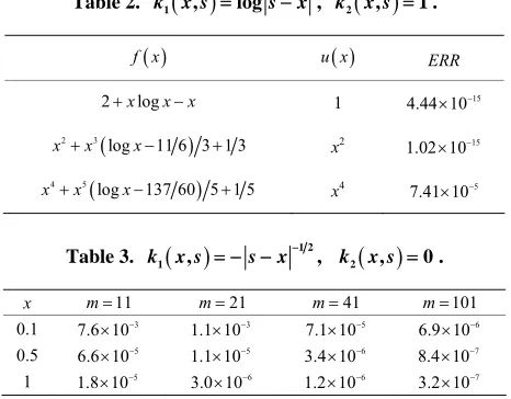
In Tables 1 and 2 we show the results obtained with

the choice k x s1

 

, k x s2

 

, s x 1 2 

    and

 

1 , log

k x s  s x , k x s2

 

, 1



 







1 1

1

1 1

n

N

I I

I



  



 _ _ _  _

 

       _ __

and we can conclude that _ I



I

 

1   _n  



1

, respectively, and λ= 1. In particular, the polynomial exactness of the method till third degree is tested.

 In the interval [0,1] we choose m11 points xj



j1, ,9



, all simple.

exists and it is bounded. Considering that from (22)











 



1

1 1

n

I

I I I



 



 



 

  _    _

 



  

 

   

The unknown function is approximated in 13 nodes belonging to

 

0,1 . For brevity in Table 1 we indicate

the mean of the absolute values of the errors evaluated in the interval.

In Table 3 we show the results obtained with the

choice 1

 

, 1 2, k x s2

 

, 0 

 k x s   s x , u x

 

 x,

 

2

f x  xx with different number of nodes in and consequently

Table 1. k₁

 

x s, k₂

 

x s,   s x1 2.  

f x u x  ERR

  3 2

2 3 1 1 2 4

x _ x  x  x _ x _{4.45 10}_ 16

 





3 _{2 7} ₁ _{1 6 5 8} 2 _{1 2} ₅ ₃₂ ₅

x  _ x  x  x  x  x7 2 _ _x3 _{9.08 10}_ 17

 





4 _{2 9} ₁ _{1 8 7 48} 2_{35 64} 3 _{1 2} ₃₅ ₂₅₆ ₃₅

(5)

[image:5.595.56.289.92.274.2]

Table 2. k1

 

x s, logsx , k2

 

x s, 1.

 

f x u x  ERR

2xlogx x 1 _{4.44 10}_ 15

 

2 3 _log _{11 6 3 1 3}

x x x  x2 _{1.02 10}_ 15

 

4 5 _log _{137 60 5 1 5}

x x x  x4 _{7.41 10}_ 5

Table 3. k1

 

x s, s x 1 2, k2

 

x s, 0



   .

x m11 21m 41m 101m 0.1 _{7.6 10}_ 3 _{1.1 10}_ 3 _{7.1 10}_ 5 _{6.9 10}_ 6

0.5 _{6.6 10}_ 5 _{1.1 10}_ 5 _{3.4 10}_ 6 _{8.4 10}_ 7

1 _{1.8 10}_ 5 _{3.0 10}_ 6 _{1.2 10}_ 6 _{3.2 10}_ 7

[0,1]. The results denote that the use of the cubic q.i. splines with a suitable densification of the nodes near using the graded mesh in [16], leads to absolute errors of the same order as the results obtained in [16] with the choice of quadratic nodal spline and the same meshes.

0,

REFERENCES

[1] T. N. E. Greville, “Spline Functions, Interpolation and Numerical Quadrature,” In: Mathematical Methods for Digital Computers, Wiley, New York, 1967, pp. 156-168. [2] C. Dagnino, “Product Integration of Singular Integrals

Based on Cubic Spline Interpolation at Equally Spaced Nodes,” Numerical Mathematics, Vol. 57, No. 1, 1990, pp. 97-104. http://dx.doi.org/10.1007/BF01386400 [3] A. P. Orsi, “Spline Approximation for Cauchy Principal

Value Integrals,” JCAM, Vol. 30, No. 1, 1990, pp. 191- 201.

[4] P. Rabinowitz, “Numerical Integration Based on Approxi-mating Splines,” Journal of Computational and Applied Mathematics, Vol. 33, No. 1, 1990, pp. 73-83.

http://dx.doi.org/10.1016/0377-0427(90)90257-Z

[5] I. J. Schoenberg, “On Spline Functions,” Inequalities (Symposium at Write-Patterson Air Force Base), Aca-demic Press, New York, 1967, pp. 255-291.

[6] T. Lyche and L. L. Schumaker, “Local Spline Approxi-mation Methods,” Journal of Approximation Theory, Vol. 15, No. 4, 1975, pp. 294-325.

http://dx.doi.org/10.1016/0021-9045(75)90091-X

[7] C. Dagnino and P. Rabinowitz, “Product Integration of Singular Integrands Using Quasi-Interpolatory Splines,”

Computers & Mathematics with Applications, Vol. 33, No. 1, 1997, pp. 59-67.

http://dx.doi.org/10.1016/S0898-1221(96)00219-2 [8] C. Dagnino and E. Santi, “Quadrature Based on Quasi-

Interpolating Spline-Projectors for Product Singular Inte-gration,” Babes-Bolyai, Mathematica, Vol. XLI, 1996, pp. 35-47.

[9] F. Caliò, E. Marchetti and P. Rabinowitz, “On the Nu-merical Solution of the Generalized Prandtl Equation Us-ing Variation-DiminishUs-ing Splines,” Journal of Computa-tional and Applied Mathematics, Vol. 60, No. 3, 1995, pp. 297-307.

http://dx.doi.org/10.1016/0377-0427(94)00024-U

[10] F. Caliò and E. Marchetti, “An Algorithm Based on q.i. Modified Splines for Singular Integral Models,” Com-puters & Mathematics with Applications, Vol. 41, No. 12, 2001, pp. 1579-1588.

http://dx.doi.org/10.1016/S0898-1221(01)00123-7 [11] F. Caliò, M. V. Fernandéz Muñoz and E. Marchetti,

“Di-rect and Iterative Methods for the Numerical Solution of Mixed Integral Equations,” Applied Mathematics and Com- putation, Vol. 216, No. 12, 2010, pp. 3739-3746.

http://dx.doi.org/10.1016/j.amc.2010.05.032

[12] F. Caliò, A. I. Garralda-Guillem, E. Marchetti and M. R. Galán, “About Some Numerical Approaches for Mixed Integral Equations,” Applied Mathematics and Computation, Vol. 219, No. 2, 2012, pp. 464-474.

http://dx.doi.org/10.1016/j.amc.2012.06.013

[13] V. Demichelis, “Quasi-Interpolatory Splines Based on Schoenberg Points,” Mathematics of Computation, Vol. 65, No. 215, 1996, pp. 1235-1247.

http://dx.doi.org/10.1090/S0025-5718-96-00728-4 [14] C. de Boor, “Spline Approximation by Quasi

Interpo-lants,” Journal of Approximation Theory, Vol. 8, No. 1, 1973, pp. 19-45.

http://dx.doi.org/10.1016/0021-9045(73)90029-4

[15] K. E. Atkinson, “The Numerical Solution of Integral Equations of the Second Kind,” Cambridge University Press, Cambridge, 1997.