Linear Plus Linear Fractional Capacitated Transportation Problem with Restricted Flow

(1)

http://dx.doi.org/10.4236/ajor.2013.36055

Linear Plus Linear Fractional Capacitated Transportation

Problem with Restricted Flow

Kavita Gupta1, Shri Ram Arora2

1_{Department of Mathematics, Ramjas College, University of Delhi, Delhi, India}

2_{Department of Mathematics, Hans Raj College, University of Delhi, Delhi, India}

Email: [email protected], srarora @yahoo.com

Received October 6, 2013; revised November 6, 2013; accepted November 13,2013

Copyright © 2013 Kavita Gupta, Shri Ram Arora. This is an open access article distributed under the Creative Commons Attribution License, which permits unrestricted use, distribution, and reproduction in any medium, provided the original work is properly cited.

Abstract

In this paper, a transportation problem with an objective function as the sum of a linear and fractional function is con- sidered. The linear function represents the total transportation cost incurred when the goods are shipped from various sources to the destinations and the fractional function gives the ratio of sales tax to the total public expenditure. Our objective is to determine the transportation schedule which minimizes the sum of total transportation cost and ratio of total sales tax paid to the total public expenditure. Sometimes, situations arise where either reserve stocks have to be kept at the supply points, for emergencies or there may be extra demand in the markets. In such situations, the total flow needs to be controlled or enhanced. In this paper, a special class of transportation problems is studied where in the total transportation flow is restricted to a known specified level. A related transportation problem is formulated and it is shown that to each basic feasible solution which is called corner feasible solution to related transportation problem, there is a corresponding feasible solution to this restricted flow problem. The optimal solution to restricted flow problem may be obtained from the optimal solution to related transportation problem. An algorithm is presented to solve a capacitated linear plus linear fractional transportation problem with restricted flow. The algorithm is supported by a real life example of a manufacturing company.

Keywords: Transportation Problem; Linear Plus Linear Fractional; Restricted Flow; Corner Feasible Solution

1. Introduction

Transportation problems with fractional objective function are widely used as performance measures in many real life situations such as the analysis of financial as- pects of transportation enterprises and undertaking, and transportation management situations, where an individ- ual, or a group of people is confronted with the hurdle of maintaining good ratios between some important and crucial parameters concerned with the transportation of commodities from certain sources to various destinations. Fractional objective function includes optimization of ratio of total actual transportation cost to total standard transportation cost, total return to total investment, ratio of risk assets to capital, total tax to total public expenditure on commodity etc. Gupta, Khanna and Puri [1] dis- cussed a paradox in linear fractional transportation problem with mixed constraints and established a sufficient condition for the existence of a paradox. Jain and Sak- sena [2] studied time minimizing transportation problem

with fractional bottleneck objective function which is solved by a lexicographic primal code. Xie, Jia and Jia [3] developed a technique for duration and cost optimization for transportation problem. In addition to this fractional objective function, if one more linear function is added, then it makes the problem more realistic. This type of objective function is called linear plus linear fractional objective function. Khuranaand Arora [4] studied linear plus linear fractional transportation problem for restricted and enhanced flow.

(2)

Many researchers like Arora and Gupta [8], Khurana, Thirwani and Arora [9] have studied restricted flow problems. Sometimes, situations arise when reserve stocks are to be kept at sources for emergencies. This gives rise to restricted flow problem where the total flow is restricted to a known specified level. This motivated us to develop an algorithm to solve a linear plus linear fractional capacitated transportation problem with restricted flow.

2. Problem Formulation

(P1): min

ij ij i I j J ij ij

i I j J ij ij i I j J

s x

z r x

t x

   

 



 



 

subject to

;

i ij i j J

a x A i I







   (1)

;

j ij j i I

b x B j J







   (2)

ij ij ij

l x u and integers  i I j, J (3)

min ,

ij i j

i I j J i I j J

x P A B

   

  

 _  _

 

 

(4)



1, 2, ,



I   m is the index set of m origins.



1, 2, ,



J  n is the index set of n destinations.

xij = number of units transported from origin i to des-

tination j.

rij = per unit transportation cost when shipment is sent

from ith_{origin to the j}th_destination.

sij = the sales tax per unit of goods transported from ith

origin to the jth_destination.

tij = the total public expenditure per unit of goods

transported from ith_{origin to the j}th_destination.

lij and uij are the bounds on number of units to be

transported from ith_{origin to j}th_destination.

ai and Ai are the bounds on the availability at the ith

origin, i  I

bj and Bj are the bounds on the demand at the jth desti-

nation, j  J

It is assumed that _ij _ij 0

i I j J t x

  

 

for every feasible

solution X satisfying (1), (2), (3) and (4) and all upper bounds uij;

 

i j,  I J are finite.

Sometimes, situations arise when one wishes to keep reserve stocks at the origins for emergencies, there by restricting the total transportation flow to a known speci-

fied level, say min _i, _j

i I j J

P A B

 

  



  

 _ _



 

. This flow con-

straint in the problem (P1) implies that a total i i I

A P



 _ 

 







of the source reserves has to be kept at the various

sources and a total _j

j I B P



 



 





 of destination slacks is to be retained at the various destinations. Therefore an extra destination to receive the source reserves and an extra source to fill up the destination slacks are intro- duced.

In order to solve the problem (P1) we convert it in to related problem (P2) given below.

(P2): min

s y

z r y

t y

 

 

 

 

 

 

 

 



 

_{ }

subject to

ij i j J

y A i I

 

 

  



ij j

i I

y B j J

 

 

  



 

, ,

ij ij ij

l y u  i j  I J

1,

0 y_m_ _j B_jb_j  j J

, 1

0 y_{i n}_ A_ia_i  i I

1, 1 0 m n

y    Ai Ai  i I

,

1

m j

j J

A _ B P



 





,

Bj Bj  j J

,

n 1 i

i I

B_ A P



 





, ,

ij ij

r r  i I jJ,

1, , 1 0 ,

m j i n

r_ r_     i I j J, r_m__1,_n_₁ M

, ,

ij ij

t t  i I jJ,

1, , 1 0 ,

m j i n

t_ t _     i I j J, t_m_{1, 1}_n  M

, ,

ij ij

s s  i I jJ,

1, , 1 0 ,

m j i n

s_ s _     i I j J ; s_m__1,_n_₁M

where M is a large positive number.



1, 2, , , 1



I   m m , J 



1, 2, , , n n1



3. Theoretical Development

Theorem1: A feasible solution 0 ij I J

X x

       



of prob-

lem (P1) with objective function value o S R

T

 



 

 



 will

be a local optimum basic feasible solution iff the following conditions holds.







 

_

_



 

2 3

1 1

3

1

0;

,

ij ij ij ij ij ij ij ij ij

ij ij ij T s z S t z r z

T T t z

i j N



 



    

 

   

 _ _ 

 

 

 

(3)







 

_

_



 

2 3 2 1 3 2 0; ,

T T t z

i j N

                 _ _         

and if X0_{is an optimal solution of (P2), then}

 

1

0; ,

ij i j N

    and 2

 

2

0; ,

ij i j N

   

where

ij ij i I j J

R r x

 



 

  _, _,

ij ij i I j J

S s x

 





 

ij ij i I j J

T t x

 



 

  _,

B denotes the set of cells (i, j) which are basic and N1 and

N2 denotes the set of non-basic cells (i, j) which are at

their lower bounds and upper bounds respectively.

1_{, , , , , ;}2 3 1 2 3 _, i i i j j j

u u u v v v iI jJ are the dual variables such that

1 1

i j ij

u v r ; ui2v2j sij;

3 3

i j ij

u v t ; 

 

i j, B;

1 1 1

i j ij

u v z ; ui2v2j zij2;

3 3 3

i j ij

u v z ; 

 

i j, B.

Proof: Let 0 ij I J X x         

be a basic feasible solution

of problem (P1) with equality constraints. Let z0_{be the}

corresponding value of objective function. Then

 











_

_



_



_



2 2 2 2

1 1 1 1

3 3 3 3

say ij ij

i I j J o

ij ij

ij i j ij i j ij

i I j J i I j J

ij i j ij i j ij

i I j J i I j J _ij _i _j _ij _i _j _ij

i I j J i I j J

s x

S

z r x R

t x T

s u v x u v x

r u v x u v x

t u v x u v x

                      _  _    _ _ _ _            

 

_{ }

 

_{ }

           









 





 





   













   









1 2 1 2 1 2

1 1 1 1 1 1

, ,

2 2 2 2 2 2

, ,

3 3 3 3 3 3

, ,

ij i j ij ij i j ij i j ij

i j N i j N i I j J

i j N i j N j J

r u v l r u v u u v x

s u v l s u v u u v x

t u v l t u v u u v x

                                        

 



  





   









   









   





1 2 1 2 1 2

1 1 1 1

, ,

2 2 2 2

, ,

3 3 3 3

, ,

i I

ij ij ij ij ij ij i i j j

i j N i j N i I j J

r z l r z u a u b v

s z l s z u a u b v

t z l t z u a u b v

                                              



 



 



 



  

Let some non-basic variable xijN1 undergoes change by an amount pq where pqis given by

 



 



min ; for all basic cells , with entry in loop;

for all basic cells , with entryin loop pq pq ij ij

ij ij

u l x l i j a

u x i j a

            

Then new value of the objective function ˆz will be given by







_

_









_

_









 

_

_



 

2 1 3 2 1 3 2 3 1 1 3 ˆ ˆ say

pq pq pq pq pq pq

pq pq pq

pq pq pq pq pq pq

pq pq pq pq pq pq pq pq

pq pq pq pq

pq pq pq

S s z

z R r z

T t z

S s z _S

z z R r z R

T

T t z

T s z S t z

r z

T T t z

(4)

Similarly, when some non-basic variable xpqN2 undergoes change by an amount pq then



1





2

 

_

_

3



2

3

ˆ o pq pq pq pq pq

pq pq pq pq

pq pq pq

T s z S t z

z z r z

T T t z



 



    

 

     

   

 

 

Hence X0_{will be local optimal solution iff}

 

1

0; ,

ij i j N

    and 2

 

2

0; ,

ij i j N

    . If X0_{is a}

global optimal solution of (P2), then it is an optimal solution and hence the result follows.

Definition: Corner feasible solution: A basic feasible

solution

 

y_ij iI,jJ to(P2) is called a corner fea-

sible solution (cfs) if y_m__1,_n_₁0

Theorem 2. A non-corner feasible solution of (P2)

cannot provide a basic feasible solution to (P1).

Proof: Let

 

yij _I___J_ be a non-corner feasible solu-

tion to (P2). Then ym1,n1

 

0

Thus

, 1 , 1 1, 1

, 1

i n i n m n

i I i I

i n i

i I i I

y y y

y  A P

    

 



 

 

   



Therefore,





, 1

i n i i I i I

y _ A P 

 

  



Now, for iI,

ij i i j J

ij i i I j J i I

y A A

y A

 



  



 

 



 



The above two relations implies that _ij

i I j J

y P 

 

 

 

This implies that total quantity transported from all the sources in I to all the destinations in J is P  P, a contradiction to the assumption that total flow is P and hence

 

yij _I_{ }__J cannot provide a feasible solution to

(P1).

Lemma1: There is a one-to-one correspondence be-

tween the feasible solution to (P1) and the corner feasible solution to (P2).

Proof: Let

 

xij _{I J}_ be a feasible solution of (P1). So

 

xij _{I J}_ will satisfy (1) to (4).

Define

 

yij _I___J_ by the following transformation

, ,

ij ij

y x iI jJ

, 1 ,

i n i ij j J

y _ A x i I



 





1, ,

m j j ij i I

y _ B x j J



 





1, 1 0

m n y _ _ 

It can be shown that

 

yij _I___J_ so defined is a cfs to

(P2)

Relation (1) to (3) implies that

for all ,

ij ij ij

l  y u iI jJ

, 1

0yi n Ai ai, iI

1,

0y_m_ _j B_j b_j, jJ

1, 1 0

m n y _ _  ,

Also for iI

, 1

ij ij i n j J j J

ij i ij i i j J j J

y y y

x A x A A

 

 

 



    



For i m 1

1, 1, 1

1

m j ij m n j ij j J j J j J i I

j ij j m

j J i I j J j J

y y y B x

B x B P A

  



   



   

 

   _  _

 



    



 



;

ij i j J

y A i I

 

 





  

Similarly, it can be shown that ij j;

i I

y B j J

 

 

  



Therefore,

 

_ij

I J y _ _

 is a cfs to (P2).

Conversely, let

 

yij _I___J_ be a cfs to (P2). Define

, ,

ij

x iI jJ by the following transformation.

, ,

ij ij

x y iI jJ

It implies that lij yij uij,iI j, J

Now for iI, the source constraints in (P2) implies

ij i i j J

y A A

 



 



, 1

ij i n i j J

y y _ A



 



i ij i j J

a y A



 



 (since 0 yi n, 1Aiai, iI).

Hence, i ij i,

j J

a x A i I







 

Similarly, for jJ, _j _ij _j

i I

b x B









For i = m + 1,

1, 1

m j m j j J j J

y _ A _ B P



 



  

(5)

1,

m j j j J j J

y _ B P

 









 (because y_m__1,_n_₁ 0)

Now, for jJ the destination constraints in (P2)

give

1,

ij m j j i I

y y _ B



 



Therefore, ij m _1,j j

i I j J j J j J

y y _ B

   

 

 



1,

ij j m j i I j J j J j J

y B y _ P

   

  

 



ij i I j J

x P

 



 



Therefore

 

_ij

I J x

 is a feasible solution to (P1)

Remark 1: If (P2) has a cfs, then since cm_1,n₁ M and d_m__1,_n_₁ M , it follows that non corner feasible

solution cannot be an optimal solution of (P2).

Lemma 2: The value of the objective function of

problem (P1) at a feasible solution

 

xij _{I J}_ is equal to

the value of the objective function of (P2) at its corresponding cfs

 

yij _I___J_ and conversely.

Proof: The value of the objective function of problem

(P2) at a feasible solution

 

yij _I___J_ is

, 1

, ,

because ij ij

ij ij

ij ij ij ij

ij ij

i I j J i I j J

ij ij ij ij

i I j J ij ij i I j J ij ij i n

i I j J i I j J

r r i I j J

s s i I j J

t t i I j J

s y s x

x y i I j J

z r y r x

t y t x r

 

   

 

    

 

   

    

     _ _{ } _

   



 _ _ _ _

  

   

   

 



 

_{ }



_

 

 

1,

, 1 1,

1, 1

0; ,

0

the value of the objective function of P1 at the corresponding feasible solution m j

i n m j

m n

ij _{I J}

r i I j J

s s i I j J

t t i I j J

y

x

      



 

 

 _ _ _{ } _ 

 

 _ _ _ _ _{ } _ 

 

       

 



 

 



The converse can be proved in a similar way.

Lemma 3: There is a one-to-one correspondence be-

tween the optimal solution to (P1) and optimal solution to the corner feasible solution to (P2).

Proof: Let ij I J x

      



be an optimal solution to (P1)

yielding objective function value z0_and

ij I J y

       



be the

corresponding cfs to (P2).Then by Lemma 2, the value yielded by _ij

I J y

       



is z0. If possible, let _ij

I J y

       



be

not an optimal solution to (P2) . Therefore, there exists a cfs

 

yij say, to (P2) with the value z

1_{< z}0_Let

 

ij x

be the corresponding feasible solution to (P1).Then by Lemma 2,

1

s x

z r x

t x

   

  

 

 



 _{ } _



 

 

 

_{ }

,

a contradiction to the assumption that _ij

I J x

      



is an op-

timal solution of (P1).Similarly, an optimal corner feasible solution to (P2) will give an optimal solution to (P1).

Theorem 3: Optimizing (P2) is equivalent to optimiz-

ing (P1) provided (P1) has a feasible solution.

Proof: As (P1) has a feasible solution, by Lemma1,

there exists a cfs to (P2). Thus by Remark 1, an optimal solution to (P2) will be a cfs. Hence, by Lemma 3, an optimal solution to (P1) can be obtained.

4. Algorithm

Step 1: Given a linear plus linear fractional capacitated

transportation problem (P1), form a related transportation problem (P2). Find a basic feasible solution of problem (P2) with respect to variable cost only. Let B be its corresponding basis.

Step 2:

Calculate ij,

1_{, , , , , , , , ;}2 3 1 2 3 1 2 3 _, i i i j j j ij ij ij

u u u v v v z z z iI jJ

such that

 

1 1 _; 2 2 _; 3 3 _, _,

i j ij i j ij i j ij

u v r u v s u v t  i j B;

 

1 1 1_; 2 2 2_; 3 3 3_, _,

i j ij i j ij i j ij

u v z u v z u v z  i j B

ij

 = level at which a non-basic cell (i,j) enters the basis replacing some basic cell of B.

1_{, , , , , ;}2 3 1 2 3 _, i i i j j j

(6)

Step 3: Calculate R S T, ,  where

, ,

ij ij ij ij ij ij

i I j J i I j J i I j J

R r x S s x T t x

     



 



 



 

  

Step 4: Find ij1;

 

i j, N1 and

 

2

; ,

ij i j N

  

where







 

_

_



 

2 3

1 1

3

1

;

,

T T t z

i j N



 



 _ _ _ 

 

  

   

 

 

 

and







 

_

_



 

2 3

2 1

3

2

;

,

T T t z

i j N



 



    

 

   

 _ _ 

 

 

 

where N1 and N2 denotes the set of non-basic cells (i,j)

which are at their lower bounds and upper bounds respectively.

If 1

 

1

0; ,

ij i j N

    and 2

 

2

0; ,

ij i j N

    then

the current solution so obtained is the optimal solution to (P2) and subsequently to (P1). Then go to step (5). Oth- erwise some

 

i j, N₁ for which  _ij1 0 or some

 

i j, N2 for which

2 ₀ ij

  will enter the basis. Go to Step 2.

Step 5: Find the optimal value of _z _Ro S T

 

_  _

 



5. Problem of the Manager of a Cell Phone

Manufacturing Company

ABC company produces cell phones. These cell phones are manufactured in the factories (i) located at Haryana, Punjab and Chandigarh. After production, these cell phones are transported to main distribution centres (j) at Kolkata, Chennai and Mumbai. The cartage paid per cell phone is 2, 3 and 4 respectively when the goods are transported from Haryana to Kolkata, Chennai and Mum- bai. Similarly, the cartage paid per cell phone when transported from Punjab to distribution centres at Kolkata, Chennai and Mumbai are 6, 1 and 2 respectively while the figures in case of transportation from Chandigarh is 1, 8 and 4 respectively. In addition to this, the company has to pay sales tax per cell phone. The sales tax paid per cell phone from Haryana to Kolkata, Chennai, Mumbai are 5, 9 and 9 respectively. The tax figures when the goods are transported from Punjab to Kolkata, Chennai and Mum- bai are 4, 6 and 2 respectively. The sales tax paid per unit from Chandigarh to Kolkata, Chennai and Mumbai are 2, 1 and 1 respectively. The total public expenditure per unit when the goods are transported from Haryana to Kolkata, Chennai and Mumbai are 4, 2 and 1 respectively

while the figures for Punjab are 3, 7 and 4. When the goods are transported from Chandigarh to distribution centres at Kolkata, Chennai and Mumbai, the total public expenditure per cell phone is 2, 9 and 4 respectively. Factory at Haryana can produce a minimum of 3 and a maximum of 30 cell phones in a month while the factory at Punjab can produce a minimum of 10 and a maximum of 40 cell phones in a month. Factory at Chandigarh can produce a minimum of 10 and a maximum of 50 cell phones in a month. The minimum and maximum monthly requirementof cell phones at Kolkata are 5 and 30 respectively while the figures for Chennai are 5 and 20 respectively and for Mumbai are 5 and 30 respectively. The bounds on the number of cell phones to be transported from Haryana to Kolkata, Chennai and Mumbai are (1, 10), (2, 10) and (0, 5) respectively. The bounds on the number of cell phones to be transported from Punjab to Kolkata, Chennai and Mumbai are (0, 15), (3, 15) and (1, 20) respectively. Thebounds on the number of cell phones to be transported from Chandigarh to Kolkata, Chennai and Mumbai are (0, 20), (0, 13) and (0, 25) respectively. The manager keeps the reserve stocks at the factories for emergencies, there by restricting the total transportation flow to 40 cell phones. He wishes to determine the number of cell phones to be shipped from each factory to different distribution centres in such a way that the total cartage plus the ratio of total sales tax paid to the total public expenditure per cell phone is minimum.

5.1. Solution

The problem of the manager can be formulated as a 3 × 3 linear plus linear fractional transportation problem (P1) with restricted flow as follows.

Let O1 and O2 and O3 denotes factories at Haryana,

Punjab and Chandigarh. D1, D2 and D3are the distribution

centres at Kolkata, Chennai and Mumbai respectively. Let the cartage be denoted by rij’s (i = 1, 2, 3 and j = 1, 2

and 3). The sales tax paid per cell phone when transported from factories (i) to distribution centres (j) is denoted by sij. The total public expenditure per cell phone

for I = 1, 2 and 3 and j = 1, 2 and 3 is denoted by tij. Then

11 12 13 21 22

23 31 32 33

2, 3, 4, 6, 1,

2, 1, 8, 4

r r r r r

r r r r

    

   

11 12 13 21 22

23 31 32 33

5, 9, 9, 4, 6,

2, 2, 1, 1

s s s s s

s s s s

    

   

11 12 13 21 22

23 31 32 33

4, 2, 1, 3, 7,

4, 2, 9, 4

t t t t t

t t t t

    

   

Let xij be the number of cell phones transported from

(7)

Since factory at Haryana can produce a minimum of 3 and a maximum of 30 cell phones in a month, it can be

formulated mathematically as 3 ₁

1

3 _j 30

j x







 .

Similarly, 3 2 3 3

1 1

10 _j 40, 10 _j 50

j j

x x

 





 



 .

Since the minimum and maximum monthly require- ment of cell phones at Kolkata are 5 and 30 respectively,

it can be formulated mathematically as 3 1 1

5 i 30

i x







 .

Similarly, 3 ₂ 3 ₃

1 1

5 _i 20, 5 _i 30.

i i

x x

 





 





The restricted flow is P = 40.

The bounds on the number of cell phones transported can be formulated mathematically as

11 12 13

1x 10, 2x 10, 0x 5,

21 22 23

0x 15, 3x 15, 1x 20,

31 32 33

0x 20, 0x 13, 0x 25

The above data can be represented in the form of Ta- ble 1 as follows.

[image:7.595.309.536.350.559.2]

Introduce a dummy source and a dummy destination in

Table 1 with

3 4

1 3 4

1

120 40 80,

80 40 40

i i

j j

B A P

A B P



    



4 4 4 0, 1, 2,3

i i i

r s t   i

and

4j 4j 4j 0, 1, 2,3

r s t   j

and

44 44 44

[image:7.595.54.286.400.718.2]

r s t M .

Table 1. Problem (P1).

D1 D2 D3 Ai

2 5 3 9 4 9 30 O1

4 2 1 6 4 1 6 2 2 40 O2

3 7 4 1 2 8 1 4 1 50 O3

2 9 4

Bj 30 20 30

Note: values in the upper left corners are rij’s and values in upper right corners

are sij’s and values in lower right corners are tij’sfor I = 1,2,3 and j = 1,2,3.

Also we have

14 24 34

41 42 43

0 27, 0 30, 0 40,

0 25, 0 15, 0 25

x x x

     

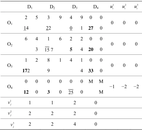
Now we find an initial basic feasible solution of prob-lem (P2) which is given in Table 2 below.

157

50 50.95

167

o o

o S R

T

   

50, 157, 167

o o o

R  S  T 

Since 1

 

1

0; ,

ij i j N

    and 2

 

2

0; ,

ij i j N

   

as shown in Table 3, the solution given in Table 2 is an

optimal solution to problem (P2) and subsequently to

(P1). Therefore min 50 157 50.94

167

o o

o S z R

T

    

Therefore, the company should send 1 cell phone from Haryana to Kolkata, 2 units from Haryana to Chennai. The number of cell phones to be shipped from factory at Punjab to Chennai and Mumbai centres are 15 and 5

Table 2. A basic feasible solution of problem (P2).

D1 D2 D3 D4 ui1

2

i

u ui3

2 5 3 9 4 9 0 0 O1

14 22 0 1 27 0 0 0 0 6 4 1 6 2 2 0 0

O2

3 15 7 5 4 20 0

0 0 0

1 2 8 1 4 1 0 0 O3

172 9 4 33 0 0 0 0

0 0 0 0 0 0 M M O4

12 0 3 0 25 0 M

−1 −2 −2

1

j

v 1 1 2 0

2

j

v 2 2 2 0

3

j

v 2 2 4 0

[image:7.595.311.537.613.736.2]

Note: Entries of the form a and b represent non basic cells which are at their lower and upper bounds respectively. Entries in bold are basic cells.

Table 3. Calculation of _ij1

and _ij2 .

NB O1D1 O1D2 O1D3 O2D1 O2D2 O3D2 O3D3 O4D3

ij

 7 3 4 7 3 3 4 3

1

ij ij

rz 1 2 2 5 0 7 2 -1

2

ij ij

s z 3 7 7 2 4 −1 −1 0

3

ij ij

t z 2 0 −3 1 5 7 0 −2

1

ij

 7.04 6.125 8.25 35.04 20.879 7.976

2

ij

(8)

respectively. Factory at Chandigarh should send 17 units to Kolkata only. The total cartage paid is 50, total sales tax paid is 157 and total public expenditure is 167.

6. Conclusion

This paper deals with a linear plus linear fractional transportation problem where in the total transportation flow is restricted to a known specified level. A related transportation problem is formulated and it is shown that it exited an optimal solution. An algorithm is presented and tested by a real life example of a manufacturing company.

7. Acknowledgements

We are thankful to the referees for their valuable com- ments with the help of which we are able to present our paper in such a nice form.

References

[1] A. Gupta, S. Khanna and M. C. Puri, “A Paradox in

Lin-ear Fractional Transportation Problems with Mixed Con-

straints,” Optimization, Vol. 27, No. 4, 1993, pp. 375-

387.

[2] M. Jain and P. K. Saksena, “Time Minimizing Transpor-

tation Problem with Fractional Bottleneck Objective

Function,” Yugoslav Journal of Operations Research, Vol.

21, No. 2, 2011, pp. 1-16.

[3] F. Xie, Y. Jia and R. Jia, “Duration and Cost Optimiza-

tion for Transportation Problem,” Advances in Informa-

tion Sciences and Service Sciences, Vol. 4, No. 6, 2012,

pp. 219-233.

[4] A. Khurana and S. R. Arora, “The Sum of a Linear and

Linear Fractional Transportation Problem with Restricted

and Enhanced Flow,” Journal of Interdisciplinary Mathe-

matics, Vol. 9, No. 9, 2006, pp. 373-383.

[5] K. Gupta and S. R. Arora, “Paradox in a Fractional Ca-

pacitated Transportation Problem,” International Journal

of Research in IT, Management and Engineering, Vol. 2, No. 3, 2012, pp. 43-64.

[6] S. Misra and C. Das, “Solid Transportation Problem with

Lower and Upper Bounds on Rim Conditions—A Note,”

New Zealand Operational Research, Vol. 9, No. 2, 1981,

pp. 137-140.

[7] S. Jain and N. Arya, “An Inverse Capacitated Transporta-

tion Problem,” IOSR Journal of Mathematics, Vol. 5, No.

4, 2013, pp. 24-27.

[8] S. R. Arora and K. Gupta, “Restricted Flow in a Non-

Linear Capacitated Transportation Problem with Bounds

on Rim Conditions,” International Journal of Manage-

ment, IT and Engineering, Vol. 2, No. 5, 2012, pp. 226-

243.

[9] A. Khurana, D. Thirwani and S. R. Arora, “An Algorithm

for Solving Fixed Charge Bi—Criterion Indefinite

Quad-ratic Transportation Problem with Restricted Flow,” In-