R E S E A R C H
Open Access
Regularized gradient-projection methods
for finding the minimum-norm solution of the
constrained convex minimization problem
Ming Tian
1,2*and Hui-Fang Zhang
1*Correspondence:
[email protected] 1College of Science, Civil Aviation
University of China, Tianjin, 300300, China
2Tianjin Key Laboratory for Advanced Signal Processing, Civil Aviation University of China, Tianjin, 300300, China
Abstract
LetHbe a real Hilbert space andCbe a nonempty closed convex subset ofH. Assume thatgis a real-valued convex function and the gradient∇gis1L-ism withL> 0. Let 0 <
λ
<L+22 , 0 <β
n< 1. We prove that the sequence{xn}generated by the iterative algorithmxn+1=PC(I–λ
(∇g+β
nI))xn,∀n≥0 converges strongly toq∈U, whereq=PU(0) is the minimum-norm solution of the constrained convex minimization problem, which also solves the variational inequality–q,p–q ≤0,∀p∈U. Under suitable conditions, we obtain some strong convergence theorems. As an application, we apply our algorithm to solving the split feasibility problem in Hilbert spaces.
MSC: 58E35; 47H09; 65J15
Keywords: regularized gradient-projection method; minimum-norm; the
constrained convex minimization problem; variational inequality
1 Introduction
LetHbe a real Hilbert space with inner product·,·and norm · . LetCbe a nonempty closed convex subset ofH. LetNandRdenote the sets of positive integers and real num-bers. Suppose thatf is a contraction onHwith coefficient <α< . A nonlinear operator T:H→His nonexpansive if Tx–Ty ≤ x–y for allx,y∈H. We useFix(T) to denote the fixed point ofT.
Firstly, consider the constrained convex minimization problem:
min
x∈Cg(x), (.)
whereg :C→Ris a real-valued convex function. Assume that the constrained con-vex minimization problem (.) is solvable, letU denote its solution set. The gradient-projection algorithm (GPA) is an effective method for solving the constrained convex min-imization problem (.). A sequence{xn}generated by the following recursive formula:
xn+=PC(I–λ∇g)xn, ∀n≥, (.)
converges strongly to a minimizer of (.). However, if the gradient∇gis only to be L-ism withL> , <λ<L, the sequence{xn}generated by (.) converges weakly to a minimizer
of (.).
Recently, many authors combined the constrained convex minimization problem with a fixed point problem [–] and proposed composited iterative algorithms to find a solution of the constrained convex minimization problem [–].
In , Moudafi [] introduced the viscosity approximation method for nonexpansive mappings.
xn+=αnf(xn) + ( –αn)Txn, ∀n≥. (.)
In , Yamada [] introduced the so-called hybrid steepest-descent algorithm:
xn+=Txn–μλnFTxn, ∀n≥, (.)
whereF is Lipschitzian and strongly monotone operator. In , Marino and Xu [] considered a generative algorithm:
xn+=αnγf(xn) + (I–αnA)Txn, ∀n≥, (.)
whereAis a strongly positive operator. In , Tian [] combined the iterative algorithm of (.), (.), and proposed a new iterative algorithm:
xn+=αnγf(xn) + (I–μαnF)Txn, ∀n≥. (.)
In , Tian [] generalized (.), obtained the following iterative algorithm:
xn+=αnγVxn+ (I–μαnF)Txn, ∀n≥, (.)
whereVis Lipschitzian operator. Based on these iterative algorithms, some authors com-bined GPA with averaged operator to solve the constrained convex minimization problem [, ].
In , Cenget al.[] proposed a sequence{xn}generated by the following iterative
algorithm:
xn+=PC
θnrh(xn) + (I–θnμF)Tn(xn)
, ∀n≥, (.)
whereh:C→His anl-Lipschitzian mapping with a constantl> , andF:C→H is ak-Lipschitzian andη-strongly monotone operator with constantsk,η> .θn=–λnL,
PC(I–λn∇g) =θnI+ ( –θn)Tn,∀n≥. Then a sequence{xn}generated by (.) converges
strongly to a minimizer of (.).
On the other hand, Xu [] proposed that regularization can be used to find the minimum-norm solution of the minimization problem.
Consider the following regularized minimization problem:
min
x∈Cgβ(x) :=g(x) +
β
x
where the regularization parameterβ> .gis a convex function and the gradient∇gis
L-ism withL> . Then the sequence{xn}generated by the following formula:
xn+=PC(I–λ∇gβn)xn=PC
I–λ(∇g+βnI)
xn, ∀n≥, (.)
where the regularization parameters <βn< , <λ<L converges weakly. But, if a
se-quence{xn}defined by
xn+=PC(I–λn∇gβn)xn=PC
I–λn(∇g+βnI)
xn, ∀n≥, (.)
where the initial guessx∈C,{λn},{βn}satisfy the following conditions:
(i) <λn≤(L+βnβn),∀n≥,
(ii) βn→(andλn→) asn→ ∞,
(iii) ∞n=λnβn=∞,
(iv) (|λn–λn–|+(λ|λnβn–λn–βn–|)
nβn) →asn→ ∞.
Then the sequence {xn} generated by (.) converges strongly to x∗, which is the
minimum-norm solution of (.) [].
Secondly, Yu et al. [] proposed a strong convergence theorem with a regularized-like method to find an element of the set of solutions for a monotone inclusion problem in a Hilbert space.
Theorem .([]) Let H be a real Hilbert space and C be a nonempty closed and convex subset of H.Let L> ,F is a L-ism mapping of C into H.Let B be a maximal monotone mapping on H and let G be a maximal monotone mapping on H such that the domains of B and G are included in C.Let Jρ= (I+ρB)–and T
r= (I+rG)–for eachρ> and r> .
Suppose that(F+B)–()∩G–()=∅.Let{x
n} ⊂H defined by
xn+=Jρ
I–ρ(F+βnI)
Trxn, ∀n> , (.)
whereρ∈(,∞),βn∈(, ),r∈(,∞).Assume that
(i) <a≤ρ< +L,
(ii) limn→∞βn= ,
∞
n=βn=∞.
Then the sequence {xn} generated by (.) converges strongly to x, where x =
P(F+B)–()∩G–()().
From the article of Yu et al. [], we obtain a new condition of parameterρ, <ρ<L+, which is used widely in our article. Motivated and inspired by Lin, when <λ<L+,{βn}
satisfy certain conditions, a sequence{xn}generated by the iterative algorithm (.):
xn+=PC
I–λ(∇g+βnI)
xn, ∀n≥,
converges strongly to a pointq∈U, whereq=PU() is the minimum-norm solution of
the constrained convex minimization problem.
2 Preliminaries
In this part, we introduce some lemmas that will be used in the rest part. LetHbe a real Hilbert space and Cbe a nonempty closed convex subset of H. We use ‘→’ to denote strong convergence of the sequence{xn}and use ‘ ’ to denote weak convergence.
RecallPCis the metric projection fromHintoC, then to each pointx∈H, the unique
pointPC∈Csatisfy the property:
x–PCx =inf
y∈C x–y =:d(x,C).
PChas the following characteristics.
Lemma .([]) For a given x∈H:
() z=PCx⇐⇒ x–z,z–y ≥,∀y∈C;
() z=PCx⇐⇒ x–z ≤ x–y – y–z ,∀y∈C;
() PCx–PCy,x–y ≥ PCx–PCy ,∀x,y∈H.
From(),we can derive that PCis nonexpansive and monotone.
Lemma .(Demiclosed principle []) Let T:C→C be a nonexpansive mapping with F(T)=∅.If{xn}is a sequence in C weakly converging to x and if {(I–T)xn} converges
strongly to y,then(I–T)x=y.In particular,if y= ,then x∈F(T).
Lemma .([]) Let{an}is a sequence of nonnegative real numbers such that
an+≤( –αn)an+αnδn, n≥,
where{αn}∞n=and{δn}∞n=are sequences of real numbers in(, )and such that
(i) ∞n=αn=∞;
(ii) lim supn→∞δn≤orn∞=αn|δn|<∞.
Thenlimn→∞an= .
3 Main results
LetHbe a real Hilbert space andCbe a nonempty closed convex subset ofH. Assume thatg:C→Ris real-valued convex function and the gradient∇g is L-ism withL> . Suppose that the minimization problem (.) is consistent and letU denote its solution set. Let <λ<L+, <βn< . Consider the following mappingGnonCdefined by
Gnx=PC
I–λ(∇g+βnI)
x, ∀x∈C,n∈N. We have
Gnx–Gny =PC
I–λ(∇g+βnI)
x–PC
I–λ(∇g+βnI)
y
≤I–λ(∇g+βnI)
x–I–λ(∇g+βnI)
y
= ( –λβn) x–y +λ∇g(x) –∇g(y)
– λ( –λβn)
x–y,∇g(x) –∇g(y)
≤( –λβn) x–y +λ∇g(x) –∇g(y)
–
Lλ( –λβn)∇g(x) –∇g(y)
≤( –λβn) x–y –λ
L( –λ) –λ
∇g(x) –∇g(y)
≤( –λβn) x–y .
That is,
Gnx–Gny ≤( –λβn) x–y .
Since < –λβn< , it follows thatGnis a contraction. Therefore, by the Banach
contrac-tion principle,Gnhas a unique fixed pointxn, such that
xn=PC
I–λ(∇g+βnI)
xn.
Next, we prove that the sequence{xn}converges strongly toq∈U, which also solves the
variational inequality
–q,p–q ≤, ∀p∈U. (.)
Equivalently,q=PU(), that is,qis the minimum-norm solution of the constrained convex
minimization problem.
Theorem . Let C be a nonempty closed convex subset of a real Hilbert space H.Let g:C→Ris real-valued convex function and assume that the gradient∇g isL-ism with L> .Assume that U=∅.Let{xn}be a sequence generated by
xn=PC
I–λ(∇g+βnI)
xn, ∀n∈N. (.)
Letλ,{βn}satisfy the following conditions:
(i) <λ<+L,
(ii) {βn} ⊂(, ),limn→∞βn= ,
∞
n=βn=∞.
Then {xn} converges strongly to a point q∈U,where q=PU(),which is the
minimum-norm solution of the minimization problem(.)and also solves the variational inequality (.).
Proof First, we claim that{xn}is bounded. Indeed, pick anyp∈U, then we have
xn–p =PC
I–λ(∇g+βnI)
xn–PC(I–λ∇g)p
≤I–λ(∇g+βnI)
xn–
I–λ(∇g+βnI)
p
+I–λ(∇g+βnI)
p– (I–λ∇g)p
≤( –λβn) xn–p +λβn p .
Then we derive that
xn–p ≤ p ,
Next, we claim that xn–PC(I–λ∇g)xn →. Indeed xn–PC(I–λ∇g)xn=PC
I–λ(∇g+βnI)
xn–PC(I–λ∇g)xn
≤I–λ(∇g+βnI)
xn– (I–λ∇g)xn
≤λβn xn .
Since{xn}is bounded,βn→ (n→ ∞), we obtain xn–PC(I–λ∇g)xn→.
∇gisL-ism. Consequently,PC(I–λ∇g) is a nonexpansive self-mapping onC. As a matter
of fact, we have for eachx,y∈C
PC(I–λ∇g)x–PC(I–λ∇g)y
≤(I–λ∇g)x– (I–λ∇g)y =x–y–λ∇g(x) –∇g(y)
= x–y – λx–y,∇g(x) –∇g(y) +λ∇g(x) –∇g(y)
≤ x–y –λ
L–λ
∇g(x) –∇g(y)
≤ x–y .
{xn}is bounded, consider a subsequence{xni}of{xn}. Since{xni}is bounded, there exists a subsequence{xnij}of{xni}which converges weakly toz. Without loss of generality, we can assume thatxni z. Then by Lemma ., we obtainz∈U.
On the other hand
xn–z =PC
I–λ(∇g+βnI)
xn–PC(I–λ∇g)z
≤I–λ(∇g+βnI)
xn– (I–λ∇g)z,xn–z
=I–λ(∇g+βnI)
xn–
I–λ(∇g+βnI)
z,xn–z
+–λβnz,xn–z
≤( –λβn) xn–z +λβn–z,xn–z.
Thus
xn–z ≤ –z,xn–z.
In particular
xni–z
≤ –z,x
ni–z.
Letqbe the minimum-norm solution ofU, that is,q=PU(). Since{xn}is bounded,
there exists a subsequence{xni}of{xn}such thatxni z. As the above proof, we know thatxni→z,z∈U.
Then we derive that
xn–q =PC
I–λ(∇g+βnI)
xn–q
≤I–λ(∇g+βnI)
xn– (I–λ∇g)q,xn–q
=I–λ(∇g+βnI)
xn–
I–λ(∇g+βnI)
q,xn–q
+–λβnq,xn–q
≤( –λβn) xn–q +λβn–q,xn–q.
Thus
xn–q ≤ –q,xn–q.
In particular
xni–q
≤ –q,x
ni–q. Sincexni→z,z∈U,
z–q ≤ –q,z–q ≤.
So, we havez=q. From the arbitrariness ofz∈U, it follows thatq∈Uis a solution of the variational inequality (.). By the uniqueness of solution of the variational inequality (.), we conclude thatxn→qasn→ ∞, whereq=PU(). Theorem . Let C be a nonempty closed convex subset of a real Hilbert space H and g:C→Ris real-valued convex function and assume that the gradient∇g isL-ism with L> .Assume that U=∅.Let{xn}be a sequence generated by x∈C and
xn+=PC
I–λ(∇g+βnI)
xn, ∀n∈N, (.)
whereλand{βn}satisfy the following conditions:
(i) <λ<L+;
(ii) {βn} ⊂(, ),limn→∞βn= ,
∞
n=βn=∞,
∞
n=|βn+–βn|<∞.
Then {xn} converges strongly to a point q∈U,where q=PU(),which is the
minimum-norm solution of the minimization problem(.)and also solves the variational inequality (.).
Proof First, we claim that{xn}is bounded. Indeed, pick anyp∈U, then we know that, for
anyn∈N,
xn+–p ≤PC
I–λ(∇g+βnI)
xn–PC
I–λ(∇g+βnI)
p
+PC
I–λ(∇g+βnI)
≤( –λβn) xn–p +λβn p
≤max xn–p , p
.
By the introduction
xn–p ≤max
x–p , p
,
and hence{xn}is bounded.
Next, we show that xn+–xn →.
xn+–xn =PC
I–λ(∇g+βnI)
xn–PC
I–λ(∇g+βn–I)
xn–
≤I–λ(∇g+βnI)
xn–
I–λ(∇g+βn–I)
xn–
=I–λ(∇g+βnI)
xn–
I–λ(∇g+βnI)
xn–
–λβnxn–+λβn–xn–
≤( –λβn) xn–xn– +λ|βn–βn–| · xn–
≤( –λβn) xn–xn– +λ|βn–βn–| ·M,
whereM=sup{ xn :n∈N}. Hence, by Lemma ., we have
xn+–xn →.
Then we claim that xn–PC(I–λ∇g)xn →.
xn–PC(I–λ∇g)xn=xn–xn++xn+–PC(I–λ∇g)xn
≤ xn–xn+ +PC
I–λ(∇g+βnI)
xn–PC(I–λ∇g)xn
≤ xn–xn+ +λβn· xn
≤ xn–xn+ +λβn·M,
sinceβn→ and xn+–xn →, we have xn–PC(I–λ∇g)xn→.
Next, we show that
lim sup
n→∞ –q,xn–q ≤. (.)
Letqbe the minimum-norm solution ofU, that is,q=PU(). Since{xn}is bounded,
without loss of generality, we assume thatxnj z. By the same argument as in the proof of Theorem ., we havez∈U.
lim sup
n→∞
–q,xn–q=lim
Then
xn+–q =PC
I–λ(∇g+βnI)
xn–PC(I–λ∇g)q
=PC
I–λ(∇g+βnI)
xn–PC
I–λ(∇g+βnI)
q,xn+–q
+PC
I–λ(∇g+βnI)
q–PC(I–λ∇g)q,xn+–q
≤( –λβn) xn–q · xn+–q +λβn–q,xn+–q
≤ –λβn
xn–q
+
xn+–q
+λβ
n–q,xn+–q.
It follows that
xn+–q ≤( –λβn) xn–q + λβn–q,xn+–q
= ( –λβn) xn–q + λβnδn,
whereδn=–q,xn+–q.
It is easy to see thatlimn→∞λβn= ,
∞
n=λβn=∞andlim supn→∞δn≤. Hence, by
Lemma ., the sequence{xn}converges strongly toq, whereq=PU(). This completes
the proof.
4 Application
In this part, we will illustrate the practical value of our algorithm in the split feasibility problem. In , Censor and Elfving [] came up with the split feasibility problem. The SFP is formulated as finding a pointxwith the property:
x∈C and Ax∈Q, (.)
whereCandQare nonempty closed and convex subset of real Hilbert spacesHandH,
A:H→His bounded linear operator.
Next, we consider the constrained convex minimization problem:
min
x∈Cg(x) =minx∈C
Ax–PQAx
. (.)
If x∗ is a solution of SFP, thenAx∗∈QandAx∗–PQAx∗= ,x∗ is the solution of the
minimization problem (.). The gradient ofgis∇g, where∇g=A∗(I–PQ)A. Applying
Theorem ., we obtain the following theorem.
Theorem . Assume that the SFP(.)is consistent.Let C be a nonempty closed convex subset of a real Hilbert space H.Assume that A:H→H is bounded linear operator,
W=∅,where W denotes the solution set of SFP(.).Let{xn}be a sequence generated by
x∈C and
xn+=PC
I–λA∗(I–PQ)A+βnI
xn, ∀n∈N. (.)
Letλand{βn}satisfy the following conditions:
(ii) {βn} ⊂(, ),limn→∞βn= ,
∞
n=βn=∞,
∞
n=|βn+–βn|<∞.
Then{xn}converges strongly to a point q∈W,where q=PW().
Proof We only need to show that∇gis A-ism, then Theorem . can be obtained by Theorem ..
∇g=A∗(I–PQ)A.
SincePQis firmly nonexpansive, soPQis-averaged mapping, thenI–PQis -ism, for
anyx,y∈C, we derive that
∇g(x) –∇g(y),x–y =A∗(I–PQ)Ax–A∗(I–PQ)Ay,x–y
=(I–PQ)Ax– (I–PQ)Ay,Ax–Ay
≥(I–PQ)Ax– (I–PQ)Ay
= A ·A
∗(I–P
Q)Ax– (I–PQ)Ay
=
A ·∇g(x) –∇g(y)
.
So,∇gis A-ism.
5 Numerical result
In this part, we use the algorithm in Theorem . to solve a system of linear equations. Then we calculate the × system of linear equations.
Example LetH=H=R. Take
A=
⎛ ⎜ ⎜ ⎜ ⎝
– – – –
–
⎞ ⎟ ⎟ ⎟
⎠, (.)
b=
⎛ ⎜ ⎜ ⎜ ⎝
– –
⎞ ⎟ ⎟ ⎟
⎠. (.)
Then the SFP can be formulated as the problem of finding a pointx∗with the property
x∗∈C and Ax∗∈Q,
whereC=R,Q={b}. That is,x∗is the solution of the system of linear equationsAx=b, and
x∗=
⎛ ⎜ ⎜ ⎜ ⎝
⎞ ⎟ ⎟ ⎟
Table 1 Numerical results as regards Example 1
n x1
n xn2 xn3 xn4 En
0 1.0000 1.0000 1.0000 1.0000 5.74E+00 100 1.2292 2.8506 1.8424 4.0887 3.28E–01 1,000 1.2208 2.9107 1.8691 4.0722 2.81E–01 5,000 1.1128 2.9543 1.9331 4.0369 1.42E–01 10,000 1.0298 2.9880 1.9824 4.0097 3.79E–02
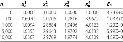
Table 2 Numerical results as regards Example 1
n x1
n xn2 xn3 xn4 En
0 1.0000 1.0000 1.0000 1.0000 3.74E+00 100 0.6070 2.0706 1.7816 3.9672 1.03E+00 1,000 1.0094 2.8884 1.9496 4.0123 1.23E–01 5,000 1.0353 2.9643 1.9702 4.0133 5.99E–02 10,000 1.0307 2.9769 1.9774 4.0109 4.59E–02
TakePC=I, whereIdenotes the × identity matrix. Given the parametersβn=(n+) forn≥,λ= . Then by Theorem ., the sequence{xn}is generated by
xn+=xn–
A
∗Ax
n+
A
∗b– (n+ )xn.
Asn→ ∞, we have{xn} →x∗= (, , , )T.
From Table , we can easily see that with iterative number increasingxnapproaches to
the exact solutionx∗and the errors gradually approach zero.
In Tian and Jiao [], they use another iterative algorithm to calculate the same example. Compare Table with Table , we find that if the parameters βnare the same, when
λ→L+, our algorithm is with fast convergence. 6 Conclusion
In a real Hilbert space, there are many methods to solve the constrained convex mini-mization problem. However, most of them cannot find the minimum-norm solution. In this article, we use the regularized gradient-projection algorithm to find the minimum-norm solution of the constrained convex minimization problem, where <λ<L+ . Then under some suitable conditions, new strong convergence theorems are obtained. Finally, we apply this algorithm to the split feasibility problem and use a concrete example and numerical results to illustrate that our algorithm has fast convergence.
Competing interests
The authors declare that they have no competing interests.
Authors’ contributions
All the authors read and approved the final manuscript.
Acknowledgements
The authors thank the referees for their helping comments, which notably improved the presentation of this paper. This work was supported by the Foundation of Tianjin Key Laboratory for Advanced Signal Processing. First author was supported by the Foundation of Tianjin Key Laboratory for Advanced Signal Processing. Hui-Fang Zhang was supported in part by Technology Innovation Funds of Civil Aviation University of China for Graduate in 2017.
[image:11.595.197.394.200.267.2]References
1. Ceng, LC, Ansari, QH, Yao, JC: Some iterative methods for finding fixed points and for solving constrained convex minimization problems. Nonlinear Anal.74, 5286-5302 (2011)
2. Ceng, LC, Ansari, QH, Yao, JC: Extragradient-projection method for solving constrained convex minimization problems. Numer. Algebra Control Optim.1(3), 341-359 (2011)
3. Ceng, LC, Ansari, QH, Wen, CF: Multi-step implicit iterative methods with regularization for minimization problems and fixed point problems. J. Inequal. Appl.2013, 240 (2013)
4. Deutsch, F, Yamada, I: Minimizing certain convex functions over the intersection of the fixed point sets of the nonexpansive mappings. Numer. Funct. Anal. Optim.19, 33-56 (1998)
5. Xu, HK: Iterative algorithms for nonlinear operators. J. Lond. Math. Soc.66, 240-256 (2002) 6. Xu, HK: An iterative approach to quadratic optimization. J. Optim. Theory Appl.116, 659-678 (2003)
7. Yamada, I, Ogura, N, Yamashita, Y, Sakaniwa, K: Quadratic approximation of fixed points of nonexpansive mappings in Hilbert spaces. Numer. Funct. Anal. Optim.19, 165-190 (1998)
8. Moudafi, A: Viscosity approximation methods for fixed-points problem. J. Math. Anal. Appl.241, 46-55 (2000) 9. Yamada, I: The hybrid steepest descent method for the variational inequality problem over the intersection of fixed
point sets of nonexpansive mappings. In: Inherently Parallel Algorithms in Feasibility and Optimization and Their Application, Haifa (2001)
10. Marino, G, Xu, HK: A general method for nonexpansive mappings in Hilbert space. J. Math. Anal. Appl.318, 43-52 (2006)
11. Tian, M: A general iterative algorithm for nonexpansive mappings in Hilbert spaces. Nonlinear Anal.73, 689-694 (2010)
12. Tian, M: A general iterative method based on the hybrid steepest descent scheme for nonexpansive mappings in Hilbert spaces. In: International Conference on Computational Intelligence and Software Engineering, CiSE 2010, art. 5677064. IEEE, Piscataway, NJ (2010)
13. Tian, M, Liu, L: General iterative methods for equilibrium and constrained convex minimization problem. Optimization63, 1367-1385 (2014)
14. Tian, M, Liu, L: Iterative algorithms based on the viscosity approximation method for equilibrium and constrained convex minimization problem. Fixed Point Theory Appl.2012, 201 (2012)
15. Xu, HK: Kim: averaged mappings and the gradient-projection algorithm. J. Optim. Theory Appl.150, 360-378 (2011) 16. Yu, ZT, Lin, LJ, Chuang, CS: A unified study of the split feasible problems with applications. J. Nonlinear Convex Anal.
15(3), 605-622 (2014)
17. Takahashi, W: Nonlinear Functional Analysis. Yokohama Publishers, Yokohama (2000)
18. Hundal, H: An alternating projection that does not converge in norm. Nonlinear Anal.57, 35-61 (2004) 19. Xu, HK: Viscosity approximation methods for nonexpansive mappings. J. Math. Anal. Appl.298, 279-291 (2004) 20. Censor, Y, Elfving, T: A multiprojection algorithm using Bregman projections in a product space. Numer. Algorithms8,
221-239 (1994)