R E S E A R C H
Open Access
A novel method of constructing
compactly supported orthogonal scaling
functions from splines
Shouzhi Yang
1and Huiqing Huang
1,2**Correspondence: [email protected] 1Department of Mathematics,
Shantou University, Shantou, Guangdong 515063, P.R. China 2School of Mathematics, Jiaying
University, Meizhou, Guangdong 514015, P.R. China
Abstract
A novel construction of compactly supported orthogonal scaling functions and wavelets with spline functions is presented in this paper. LetMnbe the center B-spline of ordern, except for the case of order one, we knowMnis not orthogonal. But by the formula of orthonormalization procedure, we can construct an orthogonal scaling function corresponding toMn. However, unlikeMnitself, this scaling function no longer has compact support. To induce the orthogonality while keeping the compact support ofMn, we put forward a simple, yet efficient construction method that uses the formula of orthonormalization procedure and the weighted average method to construct the two-scale symbol of some compactly supported orthogonal scaling functions.
Keywords: B-spline; orthogonal; compactly supported; scaling; MRA
1 Introduction
It is well known that B-splines have many useful properties, and they are widely used in practical problems. But except for the case of order one, B-splines of other orders are not orthogonal []. Thus, in order to get the property of orthogonality, many researchers are interested in the study of constructing orthogonal wavelets with B-splines [–]. For instance, Franklin wavelet and Battle-Lemarié wavelets [, ], but these wavelets are not compactly supported. In [] Goodman gave a construction, for anyn≥, of a spaceSof spline functions of degreen– with simple knots inZwhich is generated by a triple of re-finable, orthogonal functions with compact support. Subsequently, Cho and Lai simplified Goodman’s constructive steps for compactly supported orthonormal scaling functions and provided an inductive method for constructing compactly supported orthonormal wavelets []. In [] Nguyen and He presented a method to construct orthogonal spline-type scaling functions with B-splines. They multiplied a class of polynomial function fac-tors to the two-scale symbol of the B-splines so that they become the two-scale symbol of a spline-type orthogonal compactly supported function. Different from above, firstly, we use orthonormalization procedure so that splines become orthogonal scaling functions. Unfortunately, the orthogonal scaling functions are not compactly supported. So, in order to make them have the property of compact support, we use the weighted average method to eliminate the denominator of the two-scale symbol, which is the corresponding
onal scaling function. And from examples in Section , we found that this method is simple and flexible.
The goal of this section is to prepare for the next chapter of theorem proving. For this reason, we need the following auxiliary results.
Definition .([]) A Multiresolution Analysis(MRA) comprises a sequence of closed subspacesVj,j∈Z, ofL(R) satisfying
(i) (Nested)Vj⊂Vj+for allj∈Z;
(ii) (Density)j∈ZVj=L(R);
(iii) (Separation)j∈ZVj={};
(iv) (Scaling)f(x)∈Vjif and only iff(x)∈Vj+for allj∈Z;
(v) (Basis) There exists a functionφ∈Vsuch that{φ(x–k) :k∈Z}is an orthonormal
basis or a Riesz basis forV.
The functionφ defined as in Definition . is called the scaling function of the given MRA. From (iv), we know thatφ∈Vis also inV. Since{φ,k:= /φ(x–k) :k∈Z}is
a Riesz basis ofV, then there exists a uniquel-sequence{pk}satisfying the ‘two-scale
relation’
φ(x) = ∞
k=–∞
pkφ(x–k). (.)
This sequence{pk}is called the ‘two-scale sequence’ ofφ. With thisl-sequence, we define
P(ω) =
∞
k=–∞
pke–iωk. (.)
Then the Fourier transform formulation of identity (.) can be written as
φ(ω) =P
ω
φ
ω
. (.)
We callP(ω) the two-scale symbol of the scaling functionφ. Noticing that{φ(x–k) :k∈Z}
is an orthonormal basis, we have the following equivalent statements of orthogonality, see also in [, –].
Theorem . Suppose that P(ω) = kpke–iωk is a polynomial satisfying the following conditions:
P() = , (.)
P(ω) + P(ω+π) = , (.)
P(ω) > , ∀–π/ <ω<π/. (.)
Riesz lemma Let a, . . . ,aN be real numbers and aN = such that
A(ω) :=a +
N
k=
akcos(kω)≥, ∀ω∈R. (.)
Then there exists a polynomial
B(z) =
N
k=
bkzk (.)
with real coefficients and exact degree N satisfying
B(z) =A(ω), z=e–iω. (.)
2 Constructing compactly supported orthogonal scaling functions
In this section we will give a new method to construct compactly supported orthogonal scaling functions and wavelets by a center cardinal B-spline. Themth order center cardinal B-splineMmis defined as follows, see also [, ].
Mm(x) = (m– )!
m
k=
(–)k
m
k x+ m
–k
m– +
. (.)
It is well known that Mm(x) is symmetric with respect to the origin and suppMm = [–m/,m/].
Denote
m(ω) =
k∈Z
Mm(ω+ kπ) . (.)
Then, for anym≥, there exists a positive constantAmsuch that
Am≤m(ω)≤, ∀ω∈R. (.)
Furthermore, it is easy to verify that
m(ω) = – m–
k=
Mm(k)sin
kω
. (.)
Note that the scaling functionMm(x) is semi-orthogonal form≥. Next, we give a method to obtain the orthogonal scaling function through the B-splineMm. We define a functionϕm(x) through its Fourier transform
ϕm(ω) =
Mm(ω)
(k∈Z|Mm (ω+ kπ)|)/. (.)
Sincem(ω) =
k∈Z|Mm (ω+ kπ)|, then
By (.) and (.), we can obtainPm(ω),
Pm(ω) = ϕm(ω)
ϕm(ω)
=
m(ω) m(ω)
/
cosm(ω/), (.)
which is the two-scale symbol of the scaling functionϕm(x). It is well known that the
scal-ing functionϕm(x) determined by (.) is orthogonal but not compactly supported. So next
we concentrate our effort on the study of constructing compactly supported orthogonal scaling functions.
Note that the presence of the denominator in (.) can bring about scaling functions which are not compactly supported. Therefore, we multiply a function factor to the two-scale symbolPm(ω) and obtain the following Theorem . and some corollaries.
Theorem . For i= , . . . ,N,suppose that hi(ω)is the two-scale symbol of an orthogonal scaling function,and let
H(ω) =
N
i=
λi(ω) hi(ω)
, (.)
whereλi(ω)is aπ-periodic function and satisfies the following conditions:
⎧ ⎨ ⎩
≤λi(ω)≤, N
i=λi(ω) = .
Then H(ω)is the two-scale symbol of an orthogonal scaling function.
Proof It is easy to observe thatH(ω) satisfies statements (.) and (.) in Theorem ., now we only need to prove thatH(ω) also satisfies|H(ω)|+|H(ω+π)|= . Sincehi(ω)
is the two-scale symbol of an orthogonal scaling function, we have
hi(ω)
+ hi(ω+π)
= , fori= , . . . ,N.
Thus
H(ω) + H(ω+π) =
N
i=
λi(ω) hi(ω) + N
i=
λi(ω+π) hi(ω+π)
=
N
i=
λi(ω) hi(ω)
+
N
i=
λi(ω) hi(ω+π)
=
N
i=
λi(ω) = ,
which by Theorem . implies thatH(ω) is the two-scale symbol of an orthogonal scaling
Corollary . Let m≥be any integer,λ(ω) =m(ω),λ(ω) = –m(ω),Pm(ω)be defined as in(.).Suppose
Pm(ω) =
–
m–
k=
Mm(k)sin
kω
cosm(ω/)
+
m–
k=
Mm(k)sin(kω) (.)
and
Hm(ω) =λ(ω) Pm(ω)
+λ(ω) Pm(ω)
. (.)
Then Hm(ω)is a two-scale symbol of some compactly supported orthogonal scaling function.
Proof By (.) and (.), we have
Pm(ω) =
– mk=–Mm(k)sin(kω)
– mk=–Mm(k)sin(kω) /
cosm(ω/), (.)
therefore
Pm(ω)
=
– mk=–Mm(k)sin(kω)
– mk=–Mm(k)sin(kω)
cosm(ω/). (.)
SincePm(ω) is a two-scale symbol of some orthogonal scaling function, we obtain
= Pm(ω) + Pm(ω+π) = – m– k=
Mm(k)sin
kω
cosm
ω + – m– k=
Mm(k)sin
k(ω+π)
sinm
ω – m– k=
Mm(k)sin(kω)
.
Multiplying – mk=–Mm(k)sin(kω) on both sides in the above equation, we obtain
–
m–
k=
Mm(k)sin(kω)
= – m– k=
Mm(k)sin kω
cosmω + – m– k=
Mm(k)sin
k(ω+π)
it means that
=
–
m–
k=
Mm(k)sin kω
cosmω +
–
m–
k=
Mm(k)sin
k(ω+π)
sinmω
+
m–
k=
Mm(k)sin(kω). (.)
Therefore
Pm(ω)
+ Pm(ω+π)
= . (.)
By Theorem . and the Riesz lemma, we know thatHm(ω) is a two-scale symbol of some
compactly supported orthogonal scaling function.
Corollary . Let m, . . . ,mN ≥be any integer.Define hi(ω) =Pmi(ω)as in(.)and
|Pmi(ω)|
as in(.)for i= , . . . ,N.Assume that
hN+(ω) =
N
i=
Pmi(ω)
N
and
h(ω) =
N+
i=
λi(ω) hi(ω) , (.)
whereλi(ω)satisfies the following conditions:
⎧ ⎪ ⎪ ⎪ ⎪ ⎪ ⎨ ⎪ ⎪ ⎪ ⎪ ⎪ ⎩
λi(ω) =aig(ω) (i= , . . . ,N), N
i=ai(ω) = , ≤ai≤,
g(ω) =m(ω)×m(ω)× · · · ×mN(ω),
λN+(ω) = –g(ω).
Then h(ω)is the two-scale symbol of a compactly supported orthogonal scaling function.
The proof is analogous to that of Corollary ..
Corollary . Define
λ(ω) =
a+bsinω+csin(ω) – sin
ω
and
λ(ω) =
d+esinω – sin
ω–
sin
(ω)
where the real numbers a,b,c,d,e satisfy
≤a≤, b= –
a, c= –
a
, d= –a, e= a– .
Moreover,let
P(ω) =λ(ω) P(ω)
+λ(ω) P(ω)
, (.)
where P(ω)and P(ω)are defined as in(.).Then P(ω)is the two-scale symbol of a
com-pactly supported orthogonal scaling function.
To facilitate our proof of Corollary ., we need the following result.
Lemma . Define
λ(ω) =
a+bsinω+csin(ω) – sin
ω
and
λ(ω) =
d+esinω – sin
ω–
sin
(ω)
,
where a,b,c, d and e are real numbers. Then there exist real numbers a,b,c, d and e satisfying
λ(ω) +λ(ω) = . (.)
Proof By (.) we obtain
=a+d+
b–
a– d+e–
d– c
cosω+
b+
e
sinω
–
c+
e
sinω
sinω.
Now, consider the system
⎧ ⎪ ⎪ ⎪ ⎪ ⎪ ⎨ ⎪ ⎪ ⎪ ⎪ ⎪ ⎩
a+d= ,
b– a–
d+e=
b+
e,
b+ e=
d– c,
c+
e
= .
(.)
It is easy to check that the pair number (a,b,c,d,e) satisfying
b= –
a, c= –
a
, d= –a, e= a–
Lemma . Let≤x≤and≤a≤.Then
+ x+
– a x+
a – x+
–a
x+
a – x
> . (.)
Proof Define
f(a) = + x+ x
–
x
+ x–
x + – x + x – x + x
a, (.)
one obtainsf (a) = –x+x–x+x, then
⎧ ⎨ ⎩
f (a)≤, x∈[, .],
f (a)≥, x∈[., ]. (.)
Now define
⎧ ⎨ ⎩
g(x) = + x+x– x+ x–x,
g(x) = –x+x–x+x,
then
⎧ ⎨ ⎩
g(x) = +x–
x
+ x– x
,
g(x) = –x+x– x+
x.
(.)
Therefore
g(x)≥, g(x) > –., ∀x∈[, .].
This means thatf(a) > . for allx∈[, .] anda∈[, ].
Similarly, one can obtainf(a) > .×–for allx∈[., ] anda∈[, ]. This
completes the proof.
Proof of Corollary. By calculation, we have
P(ω) =
+ sinω + – a
sinω + a –
sinω
+
–a
sinω + a –
sinω
cosω .
Denote
A(ω) = + sinω + – a
sinω + a –
sinω
+
–a
sinω + a –
and note thatA(ω) is an even and π-periodic function. We obtain from Lemma .
A(ω) > , ∀ω∈R.
Therefore,|P(ω)|> .
Noticing thatP(ω) andP(ω) are the two-scale symbols of orthogonal scaling functions
andλ(ω) +λ(ω) = , we have
P(ω) + P(ω+π) = .
Now applying Theorem . and the Riesz lemma, we know thatP(ω) is a two-scale
sym-bol of some compactly supported orthogonal scaling function.
3 Examples
In this section, we give three examples to show our construction scheme introduced in the above section.
Example . Form= , from (.) and (.), we have
(ω) = –
k=
M(k)sin
kω
= – sin
ω
– sin
ω
and
P(ω) =
–sinω – sinω –sinω– sin(ω)
cos(ω/), (.)
respectively.
Moreover, we have
P(ω)
=
– sin
ω
– sin
ω
cos(ω/) + sin
ω+
sin
(ω).
Now, we obtain from (.) that
H(ω) =
– sin
ω
– sin
ω
cos(ω/) +
sin
ω+
sin
(ω)
×
– sin
ω
– sin
ω
cos(ω/) + sin
ω+
sin
(ω)
.
Therefore, by the Riesz lemma, we have
H(z) = –. – .z– .z– .z– .z
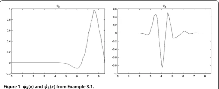
Figure 1 φ3(x) andψ3(x) from Example 3.1.
By (.) and (.) we obtain the two-scale relation
φ(x) = –.φ(x) – .φ(x– )
– .φ(x– ) – .φ(x– )
– .φ(x– ) – .φ(x– )
+ .φ(x– ) + .φ(x– )
+ .φ(x– ) + .φ(x– ),
and the corresponding wavelet
ψ(x) = .φ(x+ ) – .φ(x+ )
+ .φ(x+ ) – .φ(x+ )
– .φ(x+ ) + .φ(x+ )
– .φ(x+ ) + .φ(x+ )
– .φ(x) + .φ(x– ).
In Figure , we show the graphs ofφ(x) andψ(x), respectively.
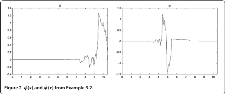
Example . Considerm= ,m= ,a=anda=, then by Corollary ., we have
h(ω) =
– sin
ω–
sin
(ω)
– sin
ω
cosω
+
– sin
ω
– sin
ω
– sin
ω
cosω
+
sin
ω+
sin
(ω) –
sin
ω–
sin
ωsin(ω)
×
– sin
ω
cosω +
sin
ω
+
– sin
ω
– sin
ω
cosω +
sin
ω+
sin
(ω)
Figure 2 φ(x) andψ(x) from Example 3.2.
Similar to the discussion of Example ., we obtainh(z),φ(x) andψ(x)
h(z) = –. + .z– .z
+ .z– .z+ .z
– .z+ .z– .z
+ .z+ .z+ .z, φ(x) = –.φ(x) + .φ(x– )
– .φ(x– ) + .φ(x– )
– .φ(x– ) + .φ(x– )
– .φ(x– ) + .φ(x– )
– .φ(x– ) + .φ(x– )
+ .φ(x– ) + .φ(x– )
and
ψ(x) = .φ(x+ ) – .φ(x+ )
+ .φ(x+ ) + .φ(x+ )
+ .φ(x+ ) + .φ(x+ )
+ .φ(x+ ) + .φ(x+ )
+ .φ(x+ ) + .φ(x+ )
+ .φ(x) + .φ(x– ),
respectively (see Figure ).
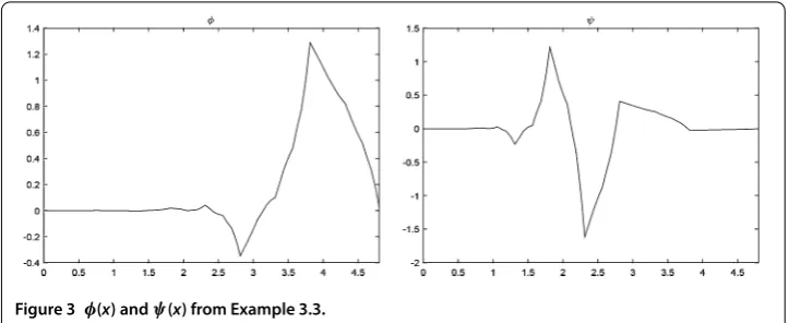
Example . Leta= , then, by Corollary .,b= –,c= ,d= –,e= . By (.), we have
P(ω) = –sinω – sin
ω
cosω –
– sin
ω
– sin
ω
Figure 3 φ(x) andψ(x) from Example 3.3.
Now from the Riesz lemma, we have
P(z) = . – .z– .z+ .z+ .z+ .z. Then we obtain from (.) and (.) the two-scale relation
φ(x) = .φ(x) – .φ(x– ) – .φ(x– ) + .φ(x– )
+ .φ(x– ) + .φ(x– ),
and the corresponding waveletψ(x) (see Figure )
ψ(x) = .φ(x+ ) – .φ(x+ ) + .φ(x+ ) + .φ(x+ )
– .φ(x) – .φ(x– ).
4 Conclusion
A simple and flexible method for constructing compactly supported orthogonal scaling functions is presented in this paper. Using this method, we can construct orthonormal compactly supported scaling functions fromB-splines. Note that the change ofλi (i=
, . . . ,N) can cause the change of the scaling functions corresponding to two-scale symbol
H(ω) in (.). Therefore we can provide the user with different scaling functions with the same compact support. Similarly, then we can obtain different compactly supported scaling functions by changing the parameters in (.).
Acknowledgements
This work was supported by the National Natural Science Foundation of China (Grant No. 11071152, 11601188), the Natural Science Foundation of Guangdong Province (Grant No. 2015A030313443).
Competing interests
The authors declare that they have no competing interests.
Authors’ contributions
All authors contributed equally to this work. All authors read and approved the final manuscript.
Publisher’s Note
Springer Nature remains neutral with regard to jurisdictional claims in published maps and institutional affiliations.
References
1. Dai, XR, Feng, DJ, Wang, Y: Structure of refinable splines. Appl. Comput. Harmon. Anal.22, 374-381 (2007) 2. Nguyen, T, He, TX: Construction of spline type orthogonal scaling functions and wavelets. J. Appl. Funct. Anal.10,
189-203 (2015)
3. He, TX: Biorthogonal spline type wavelets. Comput. Math. Appl.48, 1319-1334 (2004)
4. He, TX: Construction of biorthogonal B-spline type wavelet sequences with certain regularities. J. Appl. Funct. Anal.2, 339-360 (2007)
5. Goodman, TNT: A class of orthogonal refinable functions and wavelets. Constr. Approx.19, 525-540 (2003) 6. Cho, O, Lai, MJ: A class of compactly supported orthonormal B-spline wavelets. In: Splines and Wavelets, pp. 123-151
(2005)
7. Battle, G: A block spin construction of ondelettes, part I: Lemarié functions. Commun. Math. Phys.110, 601-615 (1987) 8. Lemarié, PG: Ondelettes a localisation exponentielles. J. Math. Pures Appl.67, 227-236 (1988)
9. Chui, CK: An Introduction to Wavelets. Wavelet Analysis and Its Applications, vol. 1. Academic Press, New York (1992) 10. Boggess, A, Narcowich, FJ: A First Course in Wavelets with Fourier Analysis. Wiley, Hoboken (2009)
11. Daubechies, I: Ten Lectures on Wavelets. CBMS-NSF Regional Conference Series in Applied Mathematics, vol. 61. SIAM, Philadelphia (1992)
12. Keinert, F: Wavelets and Multiwavelets. CRC Press, New York (2004)