2018 International Conference on Computer, Communication and Network Technology (CCNT 2018) ISBN: 978-1-60595-561-2
Modeling and Workspace Analysis of Six Degree of
Freedom Manipulator
Zhao-hui
HU*, Yu-hang ZHENG and Fan YANG
Xi’an High Technology Research Institute, Xi’an 710025, China
*Corresponding author
Keywords: D-H method, Forward kinematics, Monte carlo method, Workspace.
Abstract. Designed a 6-DOF manipulator according to this requirement. According to D-H method, the coordinate system was established for each joint of manipulator and the connecting rod parameters. Set up a kinematic model of the manipulator. Then the attitude and position of the end effector were deduced by homogeneous transformation, and the accuracy of the kinematics equation was verified by simulation and mathematical calculation. After that, according to the mapping of joint space to work space, Monte Carlo method was used to analyze the workspace of the manipulator. Finally, the 3D map of workspace was drawn in MATLAB. It provides a reference for follow-up robotic trajectory planning, motion control and parameter optimization.
Introduction
Robotics is formed by the intersection of control system theory, computer technology, structural science, sensor technology, artificial intelligence and other disciplines. Robots have very broad application prospects and are widely used in machining, assembly and welding, medical services and other fields[1].
Especially in some dangerous environments, robots can help or even replace humans to accomplish specific tasks. For example, in a radiating environment or an explosion site, the suspected explosives and radioactive contaminants can be safely transported to the designated area by the robot arm.
The robot's workspace refers to the collection of spatial points that the robot's end-effector can reach. It is one of the important indicators of robotic flexibility. At present, there are some methods for calculating robot's workspace, such as numerical method, graphical method, and analytical method. Graphical method is relatively intuitive, and can find the section and section line of the workspace, but the number of degrees of freedom can not be too much[2]. The analytical method is to perform multiple envelopes to determine the boundary of the working space. The boundaries are expressed by equations, but they are not intuitive enough, and they are only applicable to robots with few joints[3]. The numerical method can analyze any structure of the robot, the essence of which is to select enough different joint independent variable combinations, using the robot's forward kinematics equation to calculate the coordinates of the end point, the collection of these points is the workspace[4]. The greater the number of coordinate points is, the more the actual work space can be reflected.
Robot Kinematic Analysis
Establishing a Robot Kinematics Model
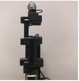
[image:2.612.108.274.182.353.2] [image:2.612.355.486.185.351.2]The robot object designed in this paper is shown in Figure 1. It is composed of a sliding joint and five rotating joints. To describe the movement relationship between the robot's adjacent bars, the robot of Figure 1 is modeled using the D-H method for kinematics modeling. The reference coordinate system for each joint of the robot is modeled. Manipulator connecting rod coordinate system was shown in Figure 2, the parameters of the table was shown in Table 1 according to the D-H method.
[image:2.612.90.523.396.498.2]Figure 1. 6-DOF robot arm. Figure 2. 6-DOF connecting rod coordinate system.
Table 1. D-H parameter table.
i
i
θ di/cm ai/cm αi range
1 90°
1
d 0 0 0~30cm
2
2
θ 7.2 0 -90° -90~90°
3
3
θ 4 30 0 -90~0°
4
4
θ -4 23 0 0~90°
5 6
5
θ
6
θ
4 25
0 0
90° 0
90~180° -90~90°
The kinematics analysis of the manipulator means that the link parameters of the manipulator and the joint angle are known, then calculate the pose of the end point relative to the reference frame. The transformation of positive kinematics is essentially a transformation from joint space to the operating space.
The transformation relationship between the robot's adjacent joint coordinate system i-1 and i is:
1 (Z , ) (0, 0, d ) (l ,1 0, 0) (X , )
i
i R i i T i T i R i i
T θ α
− = − (1)
Substituting parameters:
1 c
s c
0
0 0 0 1
i i i i i i i i i i i i i i i
i
i i i
s c s s a c
c c s a s
T
s c d
θ θ α θ α θ
θ θ α θ α θ
α α
−
−
−
=
(2)
11 12 13
21 22 23
6 1 2 3 4 5 6
0 0 1 2 3 4 5
31 32 33
0 0 0 1
x y z
r r r p
r r r p
T T T T T T T
r r r p
= = (3) The terminal's attitude vector relative to the base coordinate system is:
[
11 21 31]
T
r r r
,
[
12 22 32]
T
r r r
,
[
13 23 33]
T
r r r
,Position vector is
T x y z
p p p
.
When solving the workspace, we only focus on the position vector and get:
(
)
(
)
5 3 2 4 4 2 3 3 2 3 4 2
5 2 3 4 3 4 2 2 2 3 4
25 30 23
25 4 23
x cos cos sin sin cos sin sin cos sin cos cos sin
sin sin sin sin cos cos sin cos sin sin sin
p θ θ θ θ θ θ θ θ θ θ θ θ
θ θ θ θ θ θ θ θ θ θ θ
− + − − − − + = (4)
(
)
(
)
2 3 4 2 3 4 2 3 4 2
5 2 3 4 2 4 3 2 4 3
5
3 2
25 23 4
25 23 30
y sin cos sin sin cos cos cos cos cos cos sin
cos cos cos sin cos cos sin cos sin sin cos co
p
s
θ θ θ θ θ θ θ θ θ θ
θ θ θ θ θ θ θ θ θ θ
θ
θ θ
− − + −
+ =
− + (5)
(
)
(
)
1 25 3 4 5 23 3 4 30 3 36 / 5
z
p =d + cos θ +θ +θ − sin θ +θ − sinθ +
(6)
Verification of Robot Kinematics Model
Establishing a Robot Simulation Model. Create a robot model in MATLAB using Robotics Toolbox. The steps are as follows:
(1) According to D-H parameter table, use Link, SerialLink these two functions to create a robot object;
(2) Use the plot function to display the three-dimensional model of the robot and use the teach function to get the control panel to control each joint;
(3) Validate the created model and compare the results obtained from the simulation model with the results of homogeneous transformation matrix calculations [6].
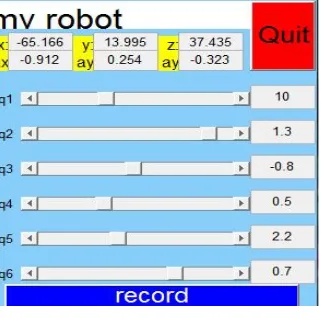
In the control panel, give any value for a set of joints: d1=10θ =2 1.3θ = −3 0.8θ =4 0.5θ =5 2.2θ =6 0.7
[image:3.612.236.403.494.653.2]The interface is shown in Figure 3, and the position vector is
[
−65.166 13.995 37.435]
T.Figure 3. Control interface of mechanical arm in MATLAB.
Substituting this set of joint values into equation (4)(5)(6), the calculated position vector is
[
−65.177 13.943 37.435]
T.Robot Workspace Analysis
The set of points in the space that the robot can reach is called the workspace. It is an important index to measure robot performance, and it is of great significance for structural design and size optimization. Regardless of the attitude of the end effector, only the position is considered and the robot's workspace is analyzed and solved.
The Monte Carlo method is a numerical method for solving approximate solutions of mathematical and engineering problems through statistical simulation of random variables and stochastic simulation. It is also called statistical simulation method. This method is simple and easy. There is no requirement for the joint type of the robot. The error is not related to the dimension. The amount of calculation is only proportional to the dimension.
The idea of using the Monte Carlo method to calculate the workspace is that each joint traverses the values within the allowable value range, and the set of end points is the workspace. Steps are as follows:
(1) Calculate the position vector P of the robot end-effector relative to the base coordinate system according to the forward kinematics equation;
(2) Within the range of the value of each joint variable, use the rand(j) function to generate N random numbers between 0 and 1, and calculate the pseudo-random value of the joint variable:
i i min ( i max i min)rand ( j)
θ =θ + θ −θ (7)
i min
θ is the minimum value of the joint variable , θi maxis the maximum value of the joint variable, i is
[image:4.612.99.483.367.682.2]the number of joints, and the value is 1~6;
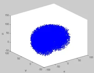
Figure 4. Workspace 3D diagram. Figure 5. Xoy plane projection.
Figure 6. Xoz plane projection. Figure 7. Yoz plane projection.
[image:4.612.111.274.370.497.2](4) The value of the obtained position vector is drawn with a sketch point to obtain the workspace of the robot.
Take N = 25000, the resulting workspace is shown in Figure 4 through Figure 7. From Figure 5, 6, and 7, the scope of the robotic workspace can be
[ 77.1407, 76.96787 ]
x∈ − cm , y∈ −[ 3.9997, 77.9294] cm,z∈ −[ 39.6029,113.6634] cm
Conclusion
(1) For the demand of manipulators under hazardous environmental conditions, design a 6-DOF manipulator first, then use the D-H method to establish a kinematics model of the manipulator, and obtain the manipulator's positive kinematics equation through homogeneous transformation. The attitude vector and position vector of the end effector are obtained, and the accuracy of the modeling is proved by the comparison of the simulation result with the mathematical calculation result.
(2) Mapping from the joint space to the workspace, the Monte Carlo method is used to calculate and describe the workspace of the robot arm by means of MATLAB. The resulting workspace is densely well-distributed and intuitive, providing a basis for follow-up trajectory planning and motion control.
References
[1]Burgard, W., et al., TelePresence in Populated Exhibitions Through Web-Operated Mobile Robots. Autonomous Robots, 2003. 15(3): p. 299-316.
[2]Abdel-Malek, K. and H.J. Yeh, Analytical Boundary of the Workspace for General3DOF Mechanisms. International Journal of Robotics Research, 1997. 16(2): p. 198-213.
[3]Botturi, D. and P. Fiorini, A Geometric Method for Robot Workspace Computation. 2003.
[4]Cao, Y., et al., Accurate Numerical Methods for Computing 2D and 3D Robot Workspace. International Journal of Advanced Robotic Systems, 2011. 8(6): p. 1-13.
[5]Jaramillo, A., Robotics Modeling and Simulation Platform. 2006.