On the Kinematic Analysis of a Spatial Six-Degree-of-Freedom Parallel Manipulator

(1)

On the Kinematic Analysis of a Spatial

Six-Degree-of-Freedom Parallel Manipulator

M. Vakil

1

_{, H. Pendar}

1

_{and H. Zohoor}

1;

Abstract. In this paper, a novel spatial six-degree-of freedom parallel manipulator actuated by three base-mounted partial spherical actuators is studied. This new parallel manipulator consists of a base platform and a moving platform, which are connected by three legs. Each leg of the manipulator is composed of a spherical joint, prismatic joint and universal joint. The base-mounted partial spherical actuators can only specify the direction of their corresponding legs. In other words, the spin of each leg is a passive degree-of-freedom. The inverse pose and forward pose of the new mechanism are described. In the inverse pose kinematics, active joint variables are calculated with no need for evaluation of the passive joint variables. To solve the forward pose problem, a much simpler method compared to the traditional method is introduced. Closed form relations for the inverse and forward rate kinematics are proposed. Finally, two sets of singular conguration of the newly introduced manipulator with dierent natures are obtained.

Keywords: Inverse kinematics; Forward kinematics; Rate kinematics; Parallel mechanism; Singular conguration.

INTRODUCTION

There have been great developments in the eld of parallel manipulators over the past decade. The par-allel manipulators have several advantages compared to serial robots, such as: high stiness, high speed, large load carrying capacity and precision positioning. However, compared to serial manipulators, parallel manipulators suer from reduced workspace and a complicated forward kinematics analysis.

Many designs of parallel manipulators with spe-cic actuation ways and Degrees-Of-Freedom (DOF) have been introduced by researchers over the past two decades. Stewart [1] designed a general six legs platform-manipulator as an airplane simulator. Hunt [2] used the Stewart platform as a robotic manip-ulator. Romiti and Sorli [3] proposed a 6-DOF parallel robot named TuPaMan. Beli [4] investigated a 6-DOF manipulator, which consisted of three PRPS legs. Hudegns and Tear [5] introduced a 6-DOF parallel ma-nipulator, in which the six inextensible legs were driven by a four-bar mechanism located on the ground.

Jong-1. Department of Mechanical Engineering, Sharif University of Technology, P.O. Box 11155-9567, Tehran, Iran.

*. Corresponding author. E-mail: [email protected]

Received 12 February 2006; received in revised form 30 Septem-ber 2007; accepted 10 March 2008

won et al. [6] presented a 6-DOF manipulator named Eclipse-II, which allowed a 360 degree spinning of the platform. Williams and Polling [7] proposed a novel 6-DOF spherically actuated platform manipulator with only two legs. There is much more research in the area of parallel manipulators [8-11]. Also, an atlas of parallel robots, created by Merlet, can be found at http: //www.inria.fr/personnel/merlet/merlet eng.html.

The novel 6-DOF manipulator studied in the present article has three legs [12]. Each leg consists of a spherical joint, a prismatic joint and universal joints (SPU). These three legs connect the equilateral moving triangle (moving platform) to the equilateral xed triangle (base platform). Each leg has a partially actuated spherical actuator. The spherical actuator of each leg can only specify the direction of the leg. Thus, the spin of the leg is a passive variable. (It is worth mentioning that each spherical actuator, if fully actuated, can specify the direction, as well as the spin, of the leg [13].) A spherical motor has been built by Lee et al. [14]. Also, there is another type of spherical motor introduced by Wang et al. [15].

The introduced manipulator here is based on the two-leg spherically actuated manipulator designed in [7], which is completely analyzed in [16]. The specic feature of the two-leg spherically actuated manipulator [7,16] is that, with only two legs, it has

(2)

6 DOF. Fewer legs lead to a smaller required space for the manipulator's installation, decrease the chance of leg collisions during maneuver and, also, mean fewer moving parts. However, the rigidity of the manipulator in [7] is not high. To increase the rigidity of the two-leg spherically actuated platform manipulator, the three-leg partially actuated spherical manipulator, as suggested in [7, p. 156], which is the subject of this research paper, is proposed [17]. Although the three-leg partially actuated spherical manipulator has an extra leg compared to the two-leg manipulator, in comparison to the other well-known 6-DOF manip-ulators, like the Stewart manipulator, it has fewer legs. Moreover, due to the existence of three spherical actuators, there are several dierent actuation ways for the manipulator, as discussed in [13]. Therefore, by combining these dierent actuation ways, it might be possible to design a singularity free parallel manipula-tor. Although, in this article, just one actuation way in which the spherical actuator species the direction of the corresponding leg is analyzed, the existence of several dierent actuation ways is another benet of the newly introduced manipulator. It is to be noted that, as discussed in [7], the SPU leg manipulator suers from a low load-carrying capacity, which is a direct consequence of its actuation. Moreover, in the presence of an external load on the moving manipulator (or even because of the weight of the platform and legs), there will be unavoidable moments on the legs. These moments should be compensated by the actuator inputs. Nonetheless, other mechanisms actuated by R-joints suer from such a deciency as well.

In this paper, the inverse and forward poses and rate kinematics of the novel mechanism are studied. In the inverse pose problem, active joint variables are calculated, with no need for evaluation of the passive joint variables. In the forward pose problem, a much simpler method compared to the traditional approach is introduced. To tackle the forward problem through the traditional approach, one has to solve twelve non-linear equations, which are obtained by equating the transformation matrices between the moving platform and the base platform through each leg. However, the new method for the forward pose problem introduced here requires the solution of only three nonlinear equations with less nonlinearity. Moreover, closed form relations for the inverse and forward rate kinematics are obtained. Finally, the singular congurations of the introduced mechanism, with their physical inter-pretations, are analyzed.

First, in the following section, the novel manipu-lator is described. Then, the inverse and forward poses, as well as the inverse and forward rate kinematics, are demonstrated. After that, the singular congurations of the mechanism are discussed. Finally, the conclusion of the research is presented.

MECHANISM AND COORDINATE DESCRIPTION

Mechanism Description

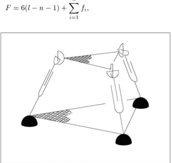
The parallel manipulator studied in the present article consists of a moving platform connected to the base platform by three legs. The moving platform and base platform are both equilateral triangles (Figure 1). Each leg is composed of a spherical joint, a prismatic joint and a universal joint, which is called a SPU leg. These joints construct each leg in a serial manner (Figure 2). Although the manipulator consists of three legs, it has 6-DOF. This is proven through the Grubler formula, as stated below:

F = 6(l n 1) +

n

X

i=1

fi;

Figure 1. Schematic of the introduced 6 DOF manipulator with three SPU legs.

Figure 2. Schematic of each SPU leg of the introduced 6 DOF manipulator.

(3)

where l is the number of links (including base), n is the number of joints, and fi is the DOF of the ith joint.

Therefore, using the Grubler formula, we have: F = 6(8 9 1) + 3(3) + 3(1) + 3(2) = 6:

The actuation of the mechanism is through the spher-ical joints and spherspher-ical actuators. The spherical actuators are partially active, since they can only specify the directions of their leg. In other words, the spin of the leg is a passive variable.

Parameters and Coordinate Description

For the base platform, as well as the moving platform, a coordinate frame is assigned. The origins of the moving platform coordinate frame and base platform coordinate frame are at the geometrical centers of the equilateral triangles, which construct the moving platform and base platform, respectively. The moving platform coordinate frame, P , base platform coordi-nate frame, B, as well as the legs' numbering, are schematically shown in Figure 3.

To specify the location and orientation of the moving platform coordinate frame, with respect to the base platform coordinate frame, the following transformation matrix is considered.

B PT =

2 6 6 4

cos() cos() cos() sin() sin() sin() cos() sin() cos() sin() sin() sin() + cos() cos()

sin() cos() sin()

0 0

cos() sin() cos() + sin() sin() x sin() sin() cos() cos() sin() y

cos() cos() z

0 1

3 7 7 5 : (1)

Figure 3. Schematic of the base and platform coordinate frames and legs' numbering.

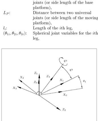
It is to be noted that the rotation part of the above transformation matrix is based on the Z Y X Euler angles. Moreover, for each leg, the standard Denavit-Hartenberg coordinate frames are assigned and the corresponding Denavit-Hartenberg parameters are obtained. In assigning the Denavit-Hartenberg coordinate frame, for each revolute and prismatic joint, a coordinate frame should be dened. If the joint is neither prismatic nor revolute, it has to be decomposed into these two base joints. For instance, the spherical joint should be decomposed into three revolute joints, in which the rotating axes of the revolute joints are mutually orthogonal to each other. A schematic of the Denavit-Hartenberg coordinate frames for a spherical joint is shown in Figure 4. In this gure, 1, 2and 3

represent the roll, yaw and pitch angles of the spherical joint.

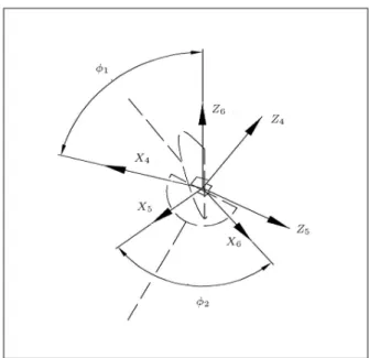
Also, the universal joint will be decomposed into two revolute joints, in such a way that the axes of the rotations of the revolute joints are orthogonal to each other. A schematic of the Denavit-Hartenberg coordinate frames for the universal joint is shown in Figure 5.

The assigned Denavit-Hartenberg coordinate frames for each leg are shown in Figure 6.

The constant platform parameters, as well as the Denavit-Hartenberg parameters for each leg of the manipulator, are as follows:

LB: Distance between two spherical

joints (or side length of the base platform),

LP: Distance between two universal

joints (or side length of the moving platform),

li: Length of the ith leg,

(1i; 2i; 3i): Spherical joint variables for the ith

leg,

Figure 4. Denavit-Hartenberg coordinate frames of the spherical joint of the SPU leg.

(4)

Figure 5. Denavit-Hartenberg coordinate frames of the universal joint of the SPU leg.

Figure 6. Denavit-Hartenberg coordinate frames of each SPU leg.

(1; 2i): Universal joint variables for the ith

leg,

In Figures 4, 5 and 6, the X and Z axes for the Denavit-Hartenberg coordinate frames are shown and the Y -axis can be easily obtained via the right-hand rule.

KINEMATICS Inverse Pose Solution

In the inverse pose procedure, the active joint variables should be calculated, havingP

BT . The active variables

for each leg are (1i; 2i)i = 1 3 and the third

spherical joint variable of each leg, ()3ii = 1 3,

is passive. The numbering of the legs is shown in Figure 3.

The transformation matrix between coordinate frame \0" and coordinate frame \6" of each leg, shown in Figure 6, can be calculated using the Denavit-Hartenberg parameters presented in Table 1. This transformation matrix is:

(0

6T )i= (01T )i(12T )i(23T )i(34T )i(45T )i(56T )i; (2)

where (k 1

kT )i is the transformation matrix between

coordinates k and k 1 of the ith leg. (0

6T )i can also

be obtained as: (0

6T )i= (B0T )i 1BPT (6PT )i1; (3)

where (B

0T )i and (6PT )i for each leg were given in the

Appendix. In the inverse kinematics, B

PT is given.

Also, (0

BT )i and (6PT )i are known, since the platform

Therefore, from Equation 3, (0

6T )i is known. Equating

the fourth column of Equations 2 and 3 leads to:

fourth column of Equation 3

z }| {

2 6 6 4

k1i

k2i

k3i

1 3 7 7

5=(B0T )i1BPT (6PT )i 1

2 6 6 4 0 0 0 1 3 7 7 5=

fourth column of Equation 2

z }| {

2 6 6 4

licos(1i) cos(2i)

lisin(1i) cos(2i)

lisin(2i)

1

3 7 7 5 :

(4) Thus, from Equation 4, the active spherical joint variables for each leg are as follows:

2i is:

2i= asin (k3i=li); (5)

and 1i is:

1i= atan 2(k2; k1) if cos(2) > 0; (6a)

1i= atan 2( k2; k1) if cos(2) < 0; (6b)

where atan 2 is the inverse tangent function considering the sign of its components and asin is the arcsin. It is worth mentioning that, for cos(2) = 0, Equations 6a

Table 1. Denavit-Hartenberg parameters for the each leg. i i 1 ai 1 di i

1 0 0 0 1

2 90 0 0 2+ 90

3 90 0 0 3

4 0 0 `f 0

5 -90 0 0 90 1

(5)

and 6b are not valid, since cos(2) = 0 leads to a

singular conguration of the mechanism, as discussed in the following sections. The active joint variables for each leg are 2i and 1i. In the following, 3i, which

is a passive variable, will be evaluated. (A reason for introducing the procedure of calculating 3here is that

this procedure will be used in the section of \Forward Pose Solution".) To calculate other passive variables, li

and 1i, 2i, an approach similar to [7] can be adopted

(See Equations 4 and 5 in [7]). Having 1i and 2i,

then, Z3i is:

B_(Z 3i) =

2

4cos(_sin(1i_1i) cos(_{) cos(2i)}2i) sin(2i)

3

5 : (7)

Also, Z6ican be derived from the third column of (06T )i,

which is:

B_(Z 6i) =

2 6 6 6 6 6 6 6 6 4

( cos(1i) sin(2i) cos(3i)

+ sin(1i) sin(3i)) cos(1i)

+ cos(1i) cos(2i) sin('1i)

( sin(1i) sin(2i) cos(3i)

cos(1i) sin(3i)) cos(1i)

+ sin(1i) cos(2i) sin(1i)

cos(2i) cos(3i) cos(1i) + sin(2i) sin(1i)

3 7 7 7 7 7 7 7 7 5 :

(8)

Cross producingB_(Z

3i) andB(Z6i), which are given in

Equations 7 and 8, respectively, results in:

B_(Z

3i) B(Z6i) =

2 6 6 6 6 6 4

cos(1i) sin(1i) cos(3i)

+ sin(2i) cos(1i) cos(1i) sin(3i)

cos(1i) cos(1i) cos(3i)

+ sin(2i) cos(1i) sin(1i) sin(3i)

cos(2i) cos(1i) sin(3i)

3 7 7 7 7 7

5: (9)

Multiplying both sides of Equation 9 by: (2

0R)i= (01R12R)i1=

2

4 _cos(cos(_1i1i_{) cos(}) sin(2i_2i)₎ _sinsin(₍1i_1i) sin(_{) cos(}2i_2i)₎ cos(_sin(2i_2i)₎

sin(1i) cos(1i) 0

3 5 ;

(10) leads to:

(2

0R)i(B(Z3i) B(Z6i)) =

2

4 sin(3i₀) cos(1i) cos(3i) cos(1i)

3 5 :

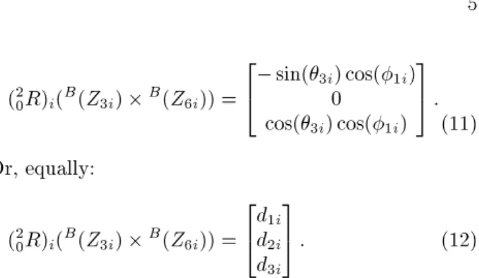
(11) Or, equally:

(2

0R)i(B(Z3i) B(Z6i)) =

2 4d_d1i_2i

d3i

3

5 : (12)

Since 1i and 2i are already calculated, B(Z3i) and

(2

0R)i are known. Also, B(Z6i), which relates to the

third column of (0

6T )i, can be obtained. Thus, the

left hand side of Equation 12 is completely known. Equating Equations 11 and 12, 3i is:

3i= atan2( d1i; d3i): (13)

It is worth noting that, if 1i= 90, then, cos(1i) = 0

and Equation 13 are not applicable. This is due to the fact that 1i= 90 leads to a singular conguration for

the introduced mechanism, as discussed in the following section. Since Equations 5 and 13 for 2i, 3iare in the

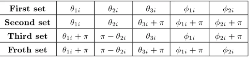
asin and atan 2 formats, it can be concluded that there are four possible sets for 1i, 2i, 3i, 1iand 2i. That

is, there are four dierent sets of 1i, 2i, 3i, 1i and

2i, which lead to the same location and orientation of

the ith leg. For example, in Figure 7, the pair (1, 2)

and the pair (1+; 2) result in the same direction

for line .

Dierent sets of 1i, 2i, 3i, 1i and 2i for the

ith leg are given in Table 2. Since there are four sets for 1, 2, 3, 1 and 2 of each, there are 64 possible sets

of 1i, 2i, 3i, 1i and 2i(i = 1 3) for the inverse

problem, which all correspond to one conguration of the mechanism.

The inverse pose problem of the introduced mech-anism is solved for the following two cases and only the rst set in Table 2 is provided. In calculating the

Figure 7. Schematic of 1, 2 of each SPU leg of the

(6)

Table 2. Multiple sets for inverse solution of the each leg. First set 1i 2i 3i 1i 2i

Second set 1i 2i 3i+ 1i+ 2i+

Third set 1i+ 2i 3i 1i 2i+

Froth set 1i+ 2i 3i+ 1i+ 2i

following variables, LP = 20 cm and LB = 30 cm were

assumed. 8 > > > > > > > > < > > > > > > > > :

x = 0 y = 5 cm z = 5 cm = 10 = 10 = 10 ) 8 > > > > > > > > > > > > > > > > > > > > > > < > > > > > > > > > > > > > > > > > > > > > > :

11= 15:93

12= 33:16

13= 16:92

21= 35:26

22= 11:98

23= 6:93

13= 56:95

23= 74:4

33= 33:16

l1= 10:5 cm

l2= 10:96 cm

l3= 7:24 cm

case I; 8 > > > > > > > > < > > > > > > > > :

x = 0 y = 5 cm z = 5 cm = 20 = 20 = 20 ) 8 > > > > > > > > > > > > > > > > > > > > > > < > > > > > > > > > > > > > > > > > > > > > > :

11= 4:69

12= 36:13

13= 35:36

21= 36:79

22= 1:25

23= 19:02

13= 55:74

23= 71:26

33= 39:45

l1= 11:13 cm

l2= 12:56 cm

l3= 9:19 cm

case II;

where x, y and z indicate the location of the origin of the moving coordinate frame, with respect to the base platform coordinate frame. Moreover, , and are the Euler angles of the moving coordinate frame, which specify its orientation. The lengths, as well as the spin, of each leg are also provided.

Forward Pose Solution

In the forward pose procedure, the location and orien-tation of the moving platform coordinate frame, with respect to the base coordinate frame, namelyB

PT , must

be obtained, having active joint variables. A traditional method to solve the forward pose of the introduced

mechanism, as adopted in [7], is to deriveB

PT through

each leg and equate them. That is: (B

PT )1= (BPT )2= (BPT )3; (14)

where (B

PT )i is obtained through the ith leg. (See

Figure 3 for the leg's numbering.) Each B

PT has six

Denavit-Hartenberg parameters, 1, 2, 3, 1, 2

and l. Since 1 and 2 are known in the forward

pose procedure, for each leg, 3, 1, 2 and l are

unknowns. Therefore, there are twelve unknowns. Also by equating two transformation matrices, six independent equations will be available. Thus, since Equation 14 leads to the following two equations, there exist twelve equations.

( (B

PT )1= (BPT )2;

(B

PT )2= (BPT )3: (15)

Therefore, twelve nonlinear equations obtained from Equation 15 must be solved for the twelve unknowns, employing numerical methods like Newton-Raphson. However, in this article, to solve the forward pose problem, a new method, diering from the traditional approach, is introduced and used. In this method, instead of solving twelve nonlinear equations, only three nonlinear equations with less nonlinearity have to be solved. Therefore, the proposed method is com-putationally more ecient. The introduced method is explained in the following. In Figure 8, the locations of the leg-platform connection points, LEP, are shown schematically.

Figure 8. Schematic of LEP points used in the forward pose solution procedure.

(7)

The coordinate for (LEP)ii = 1 3 are as

follows: The (LEP)ii = 1 3 are as follows:

(LEP)1=

2 6 6 6 6 4

0:866l1cos(11) cos(21) 0:5l1sin(11) cos(21)

0:5001LB

0:5l1cos(11) cos(21) + 0:866l1sin(11) cos(21)

0:2887LB

l1sin(21);

3 7 7 7 7 5; (LEP)2=

2 6 6 6 6 4

0:866l2cos(12) cos(22) 0:5l2sin(12) cos(22)

0:5001LB

0:5l2cos(12) cos(22) 0:866l2sin(12) cos(22)

0:2887LB

l2cos(22);

3 7 7 7 7 5;

(LEP)3=

2

4 _l₃_cos(l3₁₃sin(_{) cos(}13) cos(₂₃_{) + 0:5774L}23) _B l3sin(23)

3 5 : (16) Having 2and 1for each leg, to nd (LEP)ii = 1 3,

the length of each leg should be evaluated. Since the platform is rigid, the distance between the pair, ((LEP)i, (LEP)j), for i; j = 1 3 and i 6= j has to

always be constant and equal to lp. These restrictions

constraints result in: 8

> > > > > > < > > > > > > :

k(LEP)1(LEP)2k = LP ) l21+ l22+ 2c11l1l2

+ c21l1+ c31l2= c41

+ c22l1+ c32l3= c42

+ c23l2+ c33l3= c43

(17)

where cijfor i = 1 3; j = 1 3 are constant.

There-fore, for the forward pose problem, one can obtain l1, l2

and l3by employing a numerical method like

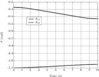
Newton-Raphson to solve Equation 17. Solving the nonlinear equations presented in Equation 17, in comparison to solving the twelve nonlinear equations derived by the traditional method, is easier and more computationally ecient. Equation 17 is solved numerically in the following for a case study. In Figures 9a, 9b and 9c, the variation of 11, 21and 12, 22 and 13, 23, with

respect to time, are shown, respectively. In Figure 10, the variations of l1, l2 and l3, with respect to time,

obtained according to the above procedure, are shown. It is to be noted that, in order to complete the forward pose problem,B

PT has to be specied, as done

in the following. Having the length and orientation of each leg, the unit vector in the direction of (X6)1,

shown in Figure 11, in the base coordinate frame, which

Figure 9a. The variations of the rst leg's active variables with respect to time in the forward pose procedure.

Figure 9b. The variations of the second leg's active variables with respect to time in the forward pose procedure.

Figure 9c. The variations of the third leg's active variables with respect to time in the forward pose procedure.

(8)

Figure 10. The variations of the lengths of the legs in the forward pose procedure.

Figure 11. Schematic of the (X6)1 used in forward pose

procedure.

is calledB_(X₆₎₁_{, is:}

B_(X 6)1=

2 6 6 6 6 6 4

x_(LEP)2+x_(LEP)3 2 y_(LEP)2+y_(LEP)3

2 z_(LEP)2+z_(LEP)3

2

3 7 7 7 7 7 5+

2 4x_y_{(LEP )}(LEP )₁1

z(LEP )1

3 5

lp p

3 2

= 2 4m_m1₂

m3

3

5 ; (18)

where x(LEP)i, y(LEP)i and z(LEP)i for i = 1 3 are

the x, y and z components of the position of (LEP)i,

respectively. The B_(X

6)1, given in Equation 18, can

be expressed in the coordinate frame by multiplying it with3

BR = (B3R) 1 as: 3_(X

6)1=3BRB(X6)1: (19)

Also, 3_(X

6)1 is equal to the rst column of (36R)1 =

(3

4R)1(45R)1(56R)1, which is: 3

6R1= (34R45R56R)1=

2

4sin(_sin(11) cos(₂₁₎ 21) sin(_cos(11) sin(₂₁₎ 21) cos(₀11) cos(11) cos(21) cos(11) sin(21) sin(11)

3 5 :

(20) Equating the rst columns of Equation 20 and 18, one has:

m = 2 4m_m1₂

m3

3 5 =3_(X

6)1=B(X6)13BR

| {z }

Completely known

= 2

4 sin(_sin(11) cos(₂₁₎ 21) cos(11) cos(21)

3 5 : So, 11is:

11= atan2(m1; m3); (21)

and 21is:

21=atan2(m2; m3= cos(11)) If 11=0 or ;

21= atan2(m2; m1= sin(11)) If 116= 0 or :

(22) After having 11 and 21, 31 must also be available

to calculate B

PT . To determine 31, the procedure

employed in previous section to calculate 3i has to

be used (see Equations 7 to 13). Finally,B PT is: B

PT = (B0T )1(03T )1(43T )1(45T )56T6PT; (23)

(B

0T )1: Known (because the location of

coordinate 0 is known); (0

3T )1: Known (because 11and 21 are inputs

and 31is specied);

(3

4T )1: Known (because `1 is calcualted);

(4

5T;56T )1: Known (bacause 11 and 21are

calcualeted); (6

PT )1: Known (because the location of

(9)

Rate Kinematics

In the inverse rate kinematics, the actuators' velocities should be calculated, having the linear velocity of the origin of the moving platform coordinate frame and the angular velocity of the moving platform. While in the forward rate kinematics, the linear velocity of the origin of the moving platform coordinate frame and the angular velocity of the moving platform should be obtained, giving the actuators' velocities.

Inverse Rate Kinematics

Before continuing, the following rule below, which will be used in this section, is introduced.

Rule I s z = ~s:z; where:

~s = 2

4 _s0_z ₀sz s_sy_x

sy sx 0

3 5 :

That is, the cross product of vector z from the left side with vector s is equivalent to per-multiplication of the skew-symmetric matrix, ~s, given above, with z.

For ease of notation and referencing, unit vectors ^n, ^x, ^h and ^x, as shown in Figure 12, are used instead of z6, z3, x5 and z5, respectively. It is to be noted that

prior to the inverse rate kinematics analysis, inverse pose kinematics are solved. Thus, all the above vectors are available.

The velocity of point LEP in Figure 12 is:

VLEP= _t + !P q; (24)

where _t is the velocity of the origin of the moving platform coordinate frame, !p is the angular velocity

Figure 12. Denition of unit vectors ^n; ^z; ^h used in the rate kinematic analysis.

of the moving platform and q is shown in Figure 12. VLEP can also be found from:

VLEP= _l^z + !l

z }| {

(! + !z) l^z; (25)

where l is the length of the leg, _l is the rate of change of the leg length, with respect to time, !l is the

leg's angular velocity, ! is the component of the leg's angular velocity along the leg's direction and !z is the

component of the leg's angular velocity, perpendicular to the leg's direction.

Equating Equations 24 and 25 and taking the dot and cross products with ^z, one obtains, respectively:

_l = ^z:VLEP; (26)

! = ^z V_lLEP: (27)

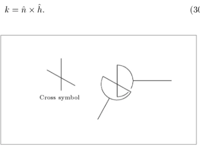
The angular velocity of the leg given in Equation 27 is perpendicular to the leg's direction. To completely dene the leg's angular velocity, its components along the leg should also be specied, as has been done below. The cross symbol of the universal joint is shown in Figure 13.

The angular velocity of the cross symbol, !CS, is:

!CS= !p+ !n; (28)

where !n is the relative angular velocity of the cross

symbol, with respect to the platform, which is in the ^n direction, and !p is the angular velocity of the

platform. Moreover, !CS is:

!CS= !l

z }| {

! + !z+ !x; (29)

where !xis the relative angular velocity of the universal

joint symbol, with respect to the leg, which is in the ^x direction. Now, dene k as:

k = ^n ^h: (30)

Figure 13. Schematic of the cross symbol of the universal joint.

(10)

Equating Equations 28 and 29 and taking the dot product of the result with k, dened in Equation 30, leads to:

k:!p= k:! + k:!z: (31)

Therefore, from Equation 31, !z is:

!z= k:(!_k:^zp !)^z: (32)

Thus, combining Equations 27 and 32, the angular velocity of the leg is:

!l= ^z V_lLEP

+

k:!p

k:^z +

k:

^z VLEP

l

1 k:^z

^z: (33)

Equation 33 can be expressed in the matrix form as: [!l] =F pv Spv _t_!

p

; F pv = ~^z_l ^z^hT

(^h:^z)l~^z; F sv = ^z^hT

^h:^z !

~^z~q l +

^z^hT

(^h:^z)l(~^z~q); (34) where the rule introduced at the beginning of this section is adopted to derived Equation 34. After having !l, then, _, _2and _3 are:

(RV ) 1₍0

BR)!l= _; (35)

where: (RV )i=

2

40₀ sin(_cos(1)₁_{) sin(}cos(₁1_{) cos(}) cos(₂2₎)

1 0 sin(2)

3 5 ;

_ = 2 4__{_}1₂

_3

3

5 ; (36)

and (0

BR) is the rotation matrix between the leg and

the base coordinate frames. Equations 34 and 36 can be used for each leg and, thus, the rate of change of the active variables, _1 and _2, will be obtained.

Due to space limitation, the result of the inverse rate kinematics is not provided here. However, the interested reader can nd the results of several inverse rate kinematic simulations in [17].

Forward Rate Kinematics

In the forward rate kinematics, _1 and _2 of each leg

are known and the platform's angular velocity and the velocity of the origin of the moving platform coordinate frame have to be obtained. Combining Equations 34 and 35, we have:

_ =

A

z }| {

(RV ) 1₍0

BR)!lF pv Spv_i _t_! p

: (37)

By considering the rst two rows of Equation 37, one obtains:

_1

_2

= A(1 : 2; 1 : 6) _t_!

p

; (38)

where A(i : j; m : n) is composed of all the components of A, which are located on the ith to jth rows and the mth to nth columns. Therefore, A(1 : 2; 1 : 6) is composed of all the components of A, which are located on the rst two rows of A (note: A has 6 columns). Equation 38 can be written for each leg and combining the equations written for the three legs leads to:

_

z }| { 2 6 6 6 6 6 6 6 4

_11

_21

_12

_22

_13

_23

3 7 7 7 7 7 7 7 5

=

B

z }| {

2

4A_A1₂(1 : 2; 1 : 6)_{(1 : 2; 1 : 6)} A3(1 : 2; 1 : 6)

3 5 _t

!p

) _ = B _t_!

p

; (39)

where Ai is the A which corresponds to the ith leg.

From Equation 39, the platform's angular velocity and the velocity of the origin of the moving platform coordinate frame are:

_t !p

= B 1_{_:} ₍₄₀₎

SINGULARITY ANALYSIS

Singular congurations for the parallel manipulators fall into two dierent major categories with dierent natures [11]. In the rst category of the singular con-gurations, the determinant of matrix B in Equation 40 is zero, while, in other categories, the determinant of matrix B approaches to innity. Conceptually, in the rst category of the singular congurations, the parallel mechanism loses one or more DOF, while, in the second category of singular congurations, it gains one or more DOF [11]. The traditional method to obtain these congurations is to derive the determinant of matrix B, and then to nd the situations in which the determinant of matrix B in Equation 39 is equal to zero or innity. However, symbolic calculation of

(11)

the determinant of matrix B results in a complicated expression. Moreover, imposing the conditions that make this determinant equal to zero or innity is not straightforward. To alleviate these drawbacks of the traditional method, in this section, the singular con-gurations of the introduced mechanism are obtained through new techniques. Also, numerical simulations available in [17] showed that, in the rst category of the singular conguration, the determinant of matrix B in Equation 40 is zero, while, in the second category of the singular conguration, this determinant approaches to innity.

First Category of the Singular Congurations This category of singular congurations represents the situations where dierent solutions can exist for the inverse kinematic. Conceptually, in this category of singular congurations, the manipulator loses one or more DOF. In another words, in this category, the mechanism reached its workspace boundary or internal boundary, limiting dierent sub regions of the workspace.

To obtain this kind of singular conguration for our introduced mechanism, rst, the Jacobian matrix of each leg should be evaluated. Having the Denavit-Hartenberg parameters for each leg from previous sections, the Jacobian Matrix and, consequently, its determinant, are calculated easily. Then, the deter-minant of the Jacobian Matrix is set to zero. The congurations that satisfy this condition will lead to the rst category of the singular congurations and the conditions to fall into this category are as follows:

det(Ji) = `2isin(2i) cos(1i);

det(J)=0) 8 < :

`i= 0 (a)

2i = 90 (b)

1i= 90 (c)

9 =

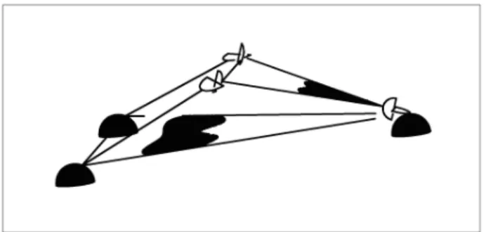
; ; (i = 1 3):₍₄₁₎ From the above equation, it is clear that there are three dierent conditions for this category of singular conguration, which are discussed in detail below. Case A `i(i = 1 3): In this case, one, or more than

one, leg(s) reaches its boundary. A schematic of the parallel manipulator at this singular conguration is shown in Figure 14. As can be seen from the schematic, the mechanism lost one DOF. It should be noted that, if, in Case A of the singular conguration, more than one leg has zero length, then, the condition lP = lB exists.

Case B 2i= 90 (i = 1 3): In this case, Z1i and

Z3i become colinear. Since the rotation axes

for 1and 3are parallel, variables 1and 3

Figure 14. Schematic of the mechanism in Case A of the rst category of the singular conguration.

act like each other. Thus, again, the mech-anism loses one DOF. Geometrically, in this case, the leg, for which the rotation axes of 1

and 3 are parallel, will be perpendicular to

the ground. A schematic of the mechanism, in this case, is shown in Figure 15. It is worth mentioning that if more than one leg wants to be perpendicular to the ground, then, the condition lP = lB exists.

Case C 1i = 90 (i = 1 3): In this case, Z6i

and Z3i become colinear and because of the

similar reason explained in Case B, again, the manipulator loses one DOF. Geometrically, in this case, the leg will be perpendicular to the moving platform. The schematic of the manipulator in this case, is shown in Figure 16. It is worth mentioning that if more than one leg wants to be perpendicular to the moving platform, then, condition lP =

lB exists.

Second Category of Singular Congurations The second category of singular congurations occurs when the platform is movable, even when the active joints are locked. Therefore, it could be easily con-cluded that, in this category, the parallel manipulator gains one or more degree of freedom. From a dierent viewpoint, this category includes the congurations of

Figure 15. Schematic of the mechanism in Case B of the rst category of the singular conguration.

(12)

Figure 16. Schematic of the mechanism in Case C of the rst category of the singular conguration.

the parallel manipulator, in which dierent solutions can exist for the forward kinematic problem. Based on the denition, as already stated, in this category, the parallel manipulator is movable, even if the actu-ators are locked. Therefore, to obtain the condition that leads to these singular congurations, rst, it is assumed that the actuators are locked and, then, the requirement that makes the manipulator movable is explored.

In Figure 17, the schematic of the parallel ma-nipulator and the angles that each leg have with the moving platform, are shown. Since the actuators are locked, points (LEP)1, (LEP)2 and (LEP)3 can only

have velocity along their corresponding leg's direction or:

V(LEP)i = _li^zi; (42)

where V(LEP)iand _liare the velocity of (LEP)iand the

derivate of li, with respect to time, respectively. Since

it is assumed that the moving platform is rigid, the

Figure 17. The schematic of the angle of the sides of the moving platform with the legs used in nding the second category of the singular conguration.

velocity given in Equation 42 is feasible, provided that the projections of V(LEP)i and V(LEP)j for i; j = 1 3,

i 6= 3 along the sides of the moving triangle that is constructed by (LEP)iand (LEP)j, be the same. These

conditions result in: 8

> < > :

_l1cos(2) _l2cos(3) = 0

_l2cos(4) _l3cos(5) = 0

_l3cos(6) _l1cos(1) = 0

(43) or:

M

z }| {

2

4 cos(₀ 2) _cos(cos(₄3₎) _cos(0 ₅₎

cos(1) 0 cos(6)

3 5=

2 4_l_{_l}1₂

_l3

3 5=

2 40₀

0 3 5 :

(44) From the above equation, if the determinant of matrix M is not equal to zero, that is, jMj 6= 0, then, the only possible solution is _li = 0 for i = 1 3. That

is, by locking the actuators, if the conguration of the manipulator is such that jMj 6= 0, then, no movement is possible. However, if the determinate of matrix M in Equation 44 is equal to zero, that is, jMj = 0, then, there can be non-zero values for _li for i = 1 3. That

is, although the actuators are locked, the platform can still move. Therefore, the manipulator will be in the second category of singular congurations if:

jMj = 0: (45)

Considering the denition of matrix M given in Equa-tion 44, the condiEqua-tion jMj = 0 is:

jMj = 0 ) cos(1) cos(3) cos(5)

= cos(2) cos(4) cos(6): (46)

From Figure 18, the following relation between cos(1),

cos(1) and cos(1) exists:

Figure 18. The schematic of the angles of the projection of each leg's extension on the moving platform.

(13)

cos(1) = cos(1) cos(1): (47)

Writing the same relation as the one given in Equa-tion 47 for cos(2), cos(3), cos(4), cos(5) and

cos(6) and substituting the results in Equation 46,

yields:

cos(1) cos(3) cos(5) = cos(2) cos(4) cos(6): (48)

Therefore, the manipulator will be in the second category of the singular conguration, provided that i for i = 1 6, as given in Figure 18, satises the

condition given in Equation 48. CONCLUSION

In this article, a new 6 Degree-Of-Freedom (DOF) parallel manipulator, which has three legs, with partial spherical actuators, was studied. Each leg of this mechanism was composed of spherical, prismatic and universal joints in a serial manner.

In the inverse pose kinematics, active joint vari-ables were calculated with no need for evaluation of the passive join variables. In the forward pose kinematics, instead of solving twelve nonlinear equations, which would have to be solved if the traditional approach were adopted, only three nonlinear equations with less nonlinearity were solved. Moreover, the inverse and forward rate kinematics were analyzed and closed form relations between actuator rates and the platform's lin-ear and angular velocities were derived. Furthermore, two dierent categories of singular congurations for mechanisms with dierent natures were introduced. In the rst category, the mechanism loses one or more DOF(s), while, in the second category, it gains one or more DOF(s).

It is clear that each spherical actuator has three inputs. Since there are three spherical joints in the mechanism, there can be up to nine independent inputs for the mechanism, while, by only six inde-pendent inputs, the location and orientation of a 6 DOF manipulator is completely specied. Thus, there are several dierent ways to actuate the introduced mechanism [13] and, in this article, only one way was studied. Assuming fully actuated spherical joints and switching from one actuation way to another would expand the mechanism workspace and might make the workspace singularity free, which can be a subject for future research.

REFERENCES

1. Stewart, D. \A platform with six degree of freedom manipulator", Proceeding of the Institute of Mechani-cal Engineering, 180(15), pp. 371-38 (1965).

2. Hunt, K.H. \Structural kinematics of in-parallel-actuated robot arms", ASME Journal of Mechanism Design, 105, pp. 705-712 (1983).

3. Romiti, A. and Sorli, M. \A parallel 6-DOF manipula-tor for cooperative work between robots in debarring", Proceeding of the 23rd International Symposium on In-dustrial Robots, Barcelona, Spain, pp. 437-442 (1992). 4. Behi, F. \Kinematics analysis for a six-degree-of-freedom 3-PRPS parallel manipulator", IEEE Trans-actions of Robotics and Automation, 4, pp. 561-565 (1988).

5. Hudgens, J. and Tear, D. \A fully-parallel six degree-of-freedom micromanipulator: Kinematics analysis and dynamic model", Proceeding of the 20th Bien-nial ASME Mechanisms Conference, 15(3), pp. 29-38 (1988).

6. Jongwon, K., Jae, H.C., Jin, K.S. and Park, F.C. \A new parallel mechanism enabling continuous 360-degree spinning plus three-axis translational motional motions", Proceeding of IEEE International Confer-ence of Robotics and Automation, Seoul, Korea, pp. 3274-3279 (2001).

7. Williams II, R.L. and Polling, D.B. \Spherically ac-tuated platform manipulator", Journal of Robotics Systems, 18(3), pp. 147-157 (2001).

8. Zhang, C.D. and Song, S.M. \Forward kinematics of a class of parallel (Stewart) platform with closed-form solution", Journal of Robotics Systems, 9(1), pp. 32-44 (1992).

9. Do, W.Q.D. and Yang, D.C.H. \Inverse dynamic analysis and simulation of a platform type robot", Journal of Robotics Systems, 5(3), pp. 209-227 (1989). 10. Daniali, H.R.M., Zsombor-Murray, P.J. and Angeles, J. \The kinematics of spatial double-triangle parallel manipulator", ASME Journal of Mechanical Design, 115(4), pp. 658-661 (1995).

11. Gosselin, C. and Angeles, J. \Singularity analysis of closed-loop kinematic chains", IEEE Transactions on Robotics and Automation, 6(3), pp. 281-290 (1990). 12. Vakil, M., Pendar, H. and Zohoor, H. \A novel

six degree-of-freedom parallel manipulator with three legs", Proceeding of the 28th ASME Biennial Mecha-nism and Robotics Conference, Salt Lake City, USA, pp. 603-610 (2004).

13. Vakil, M., Pendar, H. and Zohoor, H. \On the dierent actuation's ways of the spherically actuated platform manipulator", Proceeding of the 29th Biennial Mecha-nism and Robotics Conference, Long Beach, USA, pp. 785-792 (2005).

14. Lee, K.M., Roth, R.B. and Zhou, Z. Dynamics and Control of a Ball-Joint-Like Variable Reluctance Spherical Motor, ASME Journal of Dynamics System, Measurement and Control, 118 (1), pp. 29-40 (1996).

15. Wang, J., Wang, W., Jewell, G.W. and Hoew, D. \Novel spherical permanent magnet actuator with three degrees-of-freedom", IEEE Transactions on Magnetics, 34(4), pp. 2078-2080 (1998).

(14)

16. Pendar, H., Vakil, M., Fotouhi, R. and Zohoor, H. \Kinematic analysis of the spherically actuated plat-form manipulator", IEEE International Conference on Robotics and Automation, Roma, Italy, pp. 175-180 (2007).

17. Vakil, M. \Kinematics and dynamic analysis of the spherically actuated platform manipulator", M.S. the-sis, Sharif University of Technology, Tehran, Iran (2003).

APPENDIX (0

BT )1=

2 6 6 4

cos( 30) sin( 30) 0 Lbtg(30)

sin( 30) cos( 30) 0 0

0 0 1 0

0 0 0 1

3 7 7 5 ;

(0 BT )2=

2 6 6 4

cos( 150) sin( 150) 0 Lbtg(30)

sin( 150) cos( 150) 0 0