The alternate direction iterative methods for generalized saddle point systems

R E S E A R C H

Open Access

The alternate direction iterative methods for

generalized saddle point systems

Shuanghua Luo

_{, Angang Cui}

_{and Cheng-yi Zhang}

*_{Correspondence:}

[email protected]

3_{School of Economics and Finance,}

Xi’an Jiaotong University, Xi’an, China

Full list of author information is available at the end of the article

Abstract

The paper studies two splitting forms of generalized saddle point matrix to derive two alternate direction iterative schemes for generalized saddle point systems. Some convergence results are established for these two alternate direction iterative methods. Meanwhile, a numerical example is given to show that the proposed alternate direction iterative methods are much more effective and efficient than the existing one.

MSC: 65F10; 15A15; 15F10

Keywords: Alternate direction iterative method; Generalized saddle point system; Convergence

1 Introduction

Consider the generalized saddle-point problem

Az:=

A BT

–B 0

x y

=

f g

:=b, (1)

whereA∈Rn×n_,B∈Rm×n_,C∈Rm×m_,f∈Rn_{,f ∈R}m_andm≤n.

This class of linear systems arises in many scientific and engineering applications such as a mixed finite element approximation of elliptic partial differential equations, optimiza-tion, optimal control, structural analysis and electrical networks; see [1–11].

Recently, Benzi et al. [12,13] studied the linear systems of the form (1) whose coefficient matrix

A =

A BT

–B 0

= ⎡ ⎢ ⎣

A1 0 BT1

0 A2 BT2

–B1 –B2 0

⎤ ⎥

⎦ (2)

satisfy all of the assumptions: • A=A1 0

0 A2

,B= [B1,B2],Ai∈Rni×nifori= 1, 2andn1+n2=n, andBi∈Rm×nifor

i= 1, 2;

• Aiis positive definite (i.e., it has positive definite symmetric partHi= (Ai+ATi)/2) for

i= 1, 2; • rank(B) =m.

They [12] split the coefficient matrixA as

A =A1+A2, (3)

where

A1=

⎡ ⎢ ⎣

A1 0 BT1

0 0 0

–B1 0 0

⎤ ⎥

⎦, and A2=

⎡ ⎢ ⎣

0 0 0

0 A2 BT2

0 –B2 0

⎤ ⎥

⎦, (4)

which is called dimensional splitting ofA, and proposed the following alternate direction iterative method:

⎧ ⎨ ⎩

(αI+A1)x(k+

1

2)= (_αI–A₂)x(k)+b,

(αI+A2)x(k+1)= (αI–A1)x(k+

1 2)_+b,

(5)

which was proved to converge unconditionally for any α> 0. Meanwhile, based on di-mensional splitting ofA, they [12,13] proposed the dimensional splitting preconditioner for linear system (1), and applied a Krylov subspace method like restarted GMRES to the preconditioned linear system, and hence established some good results.

In this paper, we propose two types of alternate direction iterative methods: one is that on base of the dimensional splitting (3) the quantitative matrixαIis replaced by two non-negative diagonal matricesD1andD2to form a new alternate direction iterative scheme;

another is to propose a new splitting ofA, i.e.,

A =B1+B2, (6)

where

B1=

⎡ ⎢ ⎣

A1 0 0

0 0 BT₂

0 –B2 0

⎤ ⎥

⎦ and B2=

⎡ ⎢ ⎣

0 0 BT1

0 A2 0

–B1 0 0

⎤ ⎥

⎦, (7)

and apply the two nonnegative diagonal matrices D1 andD2 to the new splitting such

that another new alternate direction iterative scheme is obtained. Then some convergence results are established for the two alternate direction iterative schemes and a numerical example is given to show that the proposed ADI methods are much more effective and efficient than the existing one.

2 The ADI methods

In this section, two alternate direction iterative schemes are proposed based on the pre-vious two splittings (3) and (6). Let

D1=

⎡ ⎢ ⎣

0 0 0

0 αIn2 0

0 0 α₂Im

⎤ ⎥

⎦ and D2=

⎡ ⎢ ⎣

αIn1 0 0

0 0 0

0 0 α₂Im

⎤ ⎥

⎦, (8)

whereα> 0 andIm is them×midentity matrix. Then for the two splittings (3) and (6)

one has

A = (D1+A1) – (D1–A2)

= (D2+A2) – (D2–A1)

= (D1+B1) – (D1–B2)

= (D2+B2) – (D2–B1), (9)

which form the following two alternate direction iterative schemes.

Given an initial guess x(0)_{,for k= 0, 1, 2, . . . ,until{x}(k)_{}converges,compute}

⎧ ⎨ ⎩

(D1+A1)x(k+

1

2)= (D₁–A₂)x(k)+b,

(D2+A2)x(k+1)= (D2–A1)x(k+

1 2)_+b,

and (10)

⎧ ⎨ ⎩

(D1+B1)x(k+

1

2)= (D₁–B₂)x(k)+b,

(D2+B2)x(k+1)= (D2–B1)x(k+

1 2)_+b,

(11)

whereD1andD2are defined in(8).

Eliminatingx(k+1₂)_{in iterations (10) and (11), we obtain the stationary schemes}

x(k+1)=Lx(k)+f, k= 1, 2, . . . , and (12)

x(k+1)_=Tx(k)_{+g, k= 1, 2, . . . , (13)}

where

L = (D2+A2)–1(D2–A1)(D1+A1)–1(D1–A2) (14)

and

T = (D2+B2)–1(D2–B1)(D1+B1)–1(D1–B2) (15)

are the iteration matrices of the ADI iterations (12) and (13), respectively. It is easy to see that (14) and (15), respectively, are similar to the matrices

ˆ

and

ˆ

T = (D2–B1)(D1+B1)–1(D1–B2)(D2+B2)–1. (17)

As is shown in [8], the iteration matrixL is induced by the unique splittingA =P–Q withPnonsingular, i.e.,L =P–1_Q=I–P–1_{A. Furthermore,f =P}–1_{b. The matrices}

PandQare given by

P=1

α(D1+A1)(D2+A2), Q= 1

α(D2–A1)(D1–A2). (18)

Also, the iteration matrixT is induced by the unique splittingA =M–N with

M =1

α(D1+B1)(D2+B2) nonsingular, N = 1

α(D2–B1)(D1–B2), (19)

i.e.,T =M–1N =I–M–1A. Furthermore,g=M–1b. We often refer toPorM as the preconditioner.

3 The convergence of the ADI methods

In this section, some convergence results on the ADI methods will be established. First, the following lemmas will used in this section.

Lemma 1 Let A=M–N∈Cn×n_{with A and M nonsingular and let T =NM}–1_.Then A–TAT∗= (I–T)(AA–∗_M∗_+N)(I–T∗_).

The proof is similar to the proof of Lemma 5.30 in [1].

Lemma 2 Let A∈Rn×n _{be symmetric and positive definite.If A=M–N with M}

non-singular is a splitting such that M+N has a nonnegative definite symmetric part,then

TA=A–1/2TA1/22≤1,where T=NM–1. Proof It follows from Lemma1that

A–TATT= (I–T)MTA–TA+NI–TT

= (I–T)MT+NI–TT. (20)

Since

2MT+N= 2MT+M–A

=M+NT+MT+N

= (M+N) + (M+N)T

0, (21)

it follows from (20) thatA–TATT0 and thus

From (22), we haveI(A–1/2_TA1/2_)(A–1/2_TA1/2₎T_{0. Therefore,}

TA=A–1/2TA1/2₂=

ρA–1/2_TA1/2_A–1/2_TA1/2T_≤1.

This completes the proof.

Lemma 3 LetAi,BiandDibe defined in(4)and(8)for i= 1, 2.If Aihas positive definite

symmetric part Hiand0 <α≤2λmin(Hi)withλmin(Hi)the smallest eigenvalue of Hi,then

_(Dj–Ai)(Di+Ai)–1₂≤1 and (Dj–Bi)(Di+Bi)–1₂≤1, (23)

where j= 2if i= 1and j= 1if i= 2.

Proof We only prove the former inequality in (23) and the same method can yield the latter one. LetMi=Di+AiandNi= –Dj+Ai. Then we have

Ci:=Mi–Ni=Di+Dj=αdiag(In1,In1,Im) =αI0,

whereIis the (n1+n2+m)×(n1+n2+m) identity matrix, and

Mi+Ni= 2Ai+Di–Dj.

Wheni= 1 andj= 2

M1+N1= 2A1+D1–D2=

⎡ ⎢ ⎣

2A1–αIn1 0 2B

T

1

0 αIn2 0

–2B1 0 0

⎤ ⎥ ⎦.

Noting 0 <α≤2λmin(Hi), 2Hi–αIni= (A

T

i +Ai) –αIni0. Thus

(M1+N1)T+ (M1+N1)

/2 =

⎡ ⎢ ⎣

(AT

i +Ai) –αIni 0 0

0 αIn2 0

0 0 0

⎤ ⎥ ⎦0,

which shows thatM1+N1has a nonnegative definite symmetric part. Similarly,M2+N2

also has a nonnegative definite symmetric part. Thus,Mi+Nihas a nonnegative definite

symmetric part fori= 1, 2. LetTi=NiM–1i . Then it follows from Lemma2that

TiCi=C

–1/2

i TCi1/22=T2≤1.

Consequently,Ti2=NiM–1i 2=(Dj–Ai)(Di+Ai)–12≤1 fori= 1, 2. This completes

the proof.

Theorem 1 Consider problem(1)and assume that A satisfies the assumptions above.

Then A is nonsingular. Further, if 0 < α ≤2δ with δ=min{λmin(H1),λmin(H2)}, then

Proof The proof of the nonsingularity ofA can be found in [10]. Since 0 <α≤2δ= 2min{λmin(H1),λmin(H2)}, Lemma3shows that (23) hold fori= 1,j= 2 andi= 2,j= 1.

As a result,

ˆL2=(D2–A1)(D1+A1)–1(D1–A2)(D2+A2)–1₂

≤(D2–A1)(D1+A1)–1₂(D1–A2)(D2+A2)–1₂

≤1,

ˆT2=(D2–B1)(D1+B1)–1(D1–B2)(D2+B2)–1₂

≤(D2–B1)(D1+B1)–1₂(D1–B2)(D2+B2)–1₂

≤1.

(24)

This completes the proof.

Theorem 2 Consider problem(1)and assume thatA satisfies the assumptions above.If

0 <α≤2δwithδ=min{λmin(H1),λmin(H2)},then the iterations(10)and(11)are conver-gent;that is,ρ(L) < 1andρ(T) < 1.

Proof Firstly, we proveρ(L) < 1. SinceL(α) is similar toLˆ,ρ(L) =ρ(Lˆ). Letλis an eigenvalue ofLˆ(α) satisfying|λ|=ρ(Lˆ) andxis the corresponding eigenvector with x2= 1 (note that it must havex= 0). ThenLˆx=λxand consequently,

λ=x∗Lˆx=x∗(D2–A1)(D1+A1)–1(D1–A2)(D2+A2)–1x

=u∗v, (25)

whereu= (D1+A1∗)–1(D2–A1∗)xandv= (D1–A2)(D2+A2)–1x. Using the Cauchy–

Schwarz inequality,

|λ|2≤u∗u·v∗v. (26)

The equality in (26) holds if and only ifu=kv, wherek∈C. Also, Lemma3yields

u∗u=x∗(D2–A1)(D1+A1)–1

D1+A1∗

–1

D2–A1∗

x

≤ max x2=1x

∗_(D

2–A1)(D1+A1)–1

D1+A1∗

–1

D2–A1∗

x

≤(D2–A1)(D1+A1)–1 2 2

≤1,

v∗v=x∗D2+A2∗

–1

D1–A2∗

(D1–A2)(D2+A2)–1x

≤ max x2=1

x∗D2+A2∗

–1

D1–A2∗

(D1–A2)(D2+A2)–1x

≤(D1–A2)(D2+A2)–12₂

≤1.

As a result, ifu=kv, then it follows from (26) and (27) that

ρ2L(α)=ρ2Lˆ(α)=|λ|2<u∗u·v∗v≤1; (28)

ifu=kvandu∗u·v∗v< 1, then

ρ2L(α)=ρ2Lˆ(α)=|λ|2=u∗u·v∗v< 1. (29)

In what follows we will prove by contradiction thatu=kvandu∗u·v∗v= 1 do not hold simultaneously.

Assume thatu=kvandu∗u·v∗v= 1. Sinceu∗u≤1 andv∗v≤1,|k|=u∗u=v∗v= 1. Then it follows from (27) that

u∗u=x∗(D2–A1)(D1+A1)–1

D1+A1∗

–1

D2–A1∗

x

=ρ(D2–A1)(D1+A1)–1

D1+A1∗

–1

D2–A1∗

= 1,

v∗v=x∗D2+A2∗

–1

D1–A2∗

(D1–A2)(D2+A2)–1x

=ρD2+A2∗

–1

D1–A2∗

(D1–A2)(D2+A2)–1

= 1.

(30)

Noting x2= 1, (30) implies that x is the eigenvector of (D2–A1)(D1+A1)–1(D1+

A∗

1)–1(D2–A1∗) and (D2+A2∗)–1(D1–A2∗)(D1–A2)(D2+A2)–1corresponding to their

having the same eigenvalue, 1, i.e.,

(D2–A1)(D1+A1)–1

D1+A1∗

–1_D 2–A1∗

x=x,

D2+A2∗

–1

D1–A2∗

(D1–A2)(D2+A2)–1x=x.

(31)

Since

(D2–A1)(D1+A1)–1

D1+A1∗

–1_D 2–A1∗

=

⎡ ⎢ ⎣

E 0 FT

0 0 0

F 0 G

⎤ ⎥

⎦, (32)

whereE,FandGdenote nonzero matrices, the former equation in (31) can be written as

⎡ ⎢ ⎣

F 0 FT

0 0 0

F 0 G

⎤ ⎥ ⎦ ⎡ ⎢ ⎣ x1 x2 x3 ⎤ ⎥ ⎦= ⎡ ⎢ ⎣ x1 x2 x3 ⎤ ⎥ ⎦,

which indicatesx2= 0. Therefore,x= [x∗1, 0,x∗3]∗. Lety= (D2+A2)–1x. Thenx= (D2+A2)y.

The latter equation in (31) becomes

D1–A2∗

(D1–A2)y=

D2+A2∗

and consequently

D2

2–D12+α

A∗

2 +A2

y= 0, (34)

that is, ⎡ ⎢ ⎣

α2_I

n1 0 0

0 α(A∗₂+A2–αIn2) 0

0 0 0

⎤ ⎥ ⎦ ⎡ ⎢ ⎣ y1 y2 y3 ⎤ ⎥

⎦= 0, (35)

which indicatesy1= 0. Therefore,y= [0,y∗2,y3∗]∗. Also,x= (D2+A2)y. Then

⎡ ⎢ ⎣ x1 0 x3 ⎤ ⎥ ⎦= ⎡ ⎢ ⎣

αIn1 0 0

0 A2 BT2

0 –B2 α₂Im

⎤ ⎥ ⎦ ⎡ ⎢ ⎣ 0 y2 y3 ⎤ ⎥ ⎦= ⎡ ⎢ ⎣ 0

A2y2+BT2y3

–B2y2+α₂y3

⎤ ⎥

⎦, (36)

which shows that

x1=y1= 0, A2y2+B2Ty3= 0, and x3= –B2y2+ α

2y3. (37)

Sinceu=kv,

D1+A1∗

–1

D2–A1∗

x=k(D1–A2)(D2+A2)–1x, (38)

which can be written as

D2–A1∗

(D2+A2)y=k

D1+A1∗

(D1–A2)y (39)

forx= (D2+A2)y. Further, (39) becomes

D2

2 –kD12

+ (D2+kD1)A2–A1∗(D2+kD1) – (1 –k)A1∗A2

y= 0, (40)

i.e., ⎡ ⎢ ⎣

α2_I

n1–αA∗1 (k– 1)B1BT2 (1+k)

α

2 BT1

0 kα(A2–αIn2) kαBT2

–αB1 –(1+₂k)αB1 (1–k)α

2

4 Im

⎤ ⎥ ⎦ ⎡ ⎢ ⎣ 0 y2 y3 ⎤ ⎥ ⎦= ⎡ ⎢ ⎣ 0 0 0 ⎤ ⎥

⎦, (41)

i.e., ⎧ ⎪ ⎪ ⎨ ⎪ ⎪ ⎩

(k– 1)B1BT2y2+(1+₂k)αBT1y3= 0, kα(A2–αIn2)y2+kαBT2y3= 0,

–(1+₂k)αB1y2+(1–k)α

2

4 y3= 0.

(42)

Here, we assertk= 1. Otherwise, assumek= 1. Then (25) showsλ=u∗v=v∗v= 1 for

be the eigenvector ofL corresponding to the eigenvalue 1 (note that necessarilyw= 0).

One has

Lw=(D1+A1)(D2+A2)

–1_(D

2–A1)(D1–A2)

w=w (43)

and consequently

(D2–A1)(D1–A2) – (D1+A1)(D2+A2)

w= –αAw= 0. (44)

SinceA is nonsingular, (44) yieldsw= 0, which contradicts thatwis an eigenvector of L(α). Thus,k= 1 and 1 –k= 0. From the third equation in (42), one has

y3=κB1y2 (45)

withκ:=_α2(1+_(1–k_k)₎. Then it follows from the second equation in (37) that Jy2=

A2+κBT1B1

y2= 0, (46)

whereJ=A2+κBT1B1. Note|k|= 1 andk= 1. Letk=cosθ+isinθ, wherei=

√

–1,θ∈R, θ= 2tπandtis an integer. Then

κ:=2(1 +k) α(1 –k)=

2[(1 +cosθ) +isinθ] α[(1 –cosθ) –isinθ]=

2i

α tan θ

2 (47)

is either pure imaginary or zero. As a result,J∗+J =A₂T+A20 forA2 is positive

definite. Thus,Jis positive definite and hence nonsingular. Equation (46) indicatesy2= 0

and thus (45) shows thaty3= 0. Then it follows from the third equation in (37) thatx3= 0.

Therefore,x= [0, 0, 0]∗, which contradicts thatxis an eigenvector ofLˆ(α) withx2= 1.

By the proof above, it is easy to see thatu=kvandu∗u·v∗v= 1 do not hold simultaneously. Therefore,ρ[L(α)] =|λ|< 1 and consequently, the iteration (10) converges.

By the same method, we can obtainρ(T) < 1. Therefore, iterations (10) and (11) are

both convergent. This completes the proof.

4 A numerical example

A numerical example is given in this section to show that the proposed alternate direction iterative methods are very effective.

Example1 Consider problem (1) and assume thatA is shown in (2), whereA1=A2=

tri(1, 1, –1)∈Rn×n,B1=B2=In∈Rn×n, ann×nidentity matrix andb= (1, 1, . . . , 1)T∈R2n.

Table 1 Performance of A1, A2, and A3 with differentn

Algorithm n RE k Time (s)

A1 500 9.97e–07 263 1.05

1000 9.56e–07 260 10.38

1500 9.47e–07 261 34.12

A2 500 8.99e–07 17 0.69

1000 9.03e–07 17 5.13

1500 9.17e–07 17 23.77

A3 500 9.29e–07 126 0.63

1000 9.69e–07 126 4.37

1500 9.90e–07 125 12.18

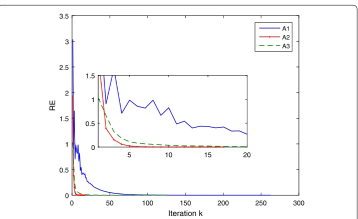
Figure 1Whenn= 1000 the change of RE of A1, A2 and A3 with the iteration number increasing

The stopping criterion is defined as

RERE = x

k+1_–xk

2

max{1,xk

2}

=< 10–6.

Numerical results are presented in Table1. In particular, we report in Fig.1the change of RE of A1, A2 and A3 whenn= 1000 with the iteration number increasing.

From Table1, we can make the following observations. (i) A2 (i.e., Algorithm 2) gener-ally has much smaller iteration number than A1 and A3 (Algorithm 1 and Algorithm 3) whenn= 500,n= 1000 andn= 1500; (ii) A3 has much less computing time than A2 and A1. Thus, both A2 and A3 are generally superior to A1 in terms of iteration number and computing time. Therefore, the proposed methods are more effective and efficient than the existing method.

5 Conclusions

In this paper we propose two alternate direction iterative methods for generalized saddle-point systems based on two splitting forms of generalized saddle-saddle-point matrix, and then establish some convergence theorems for these two iterative methods. Finally, we present a numerical example to demonstrate that the proposed alternate direction iterative methods are superior to the existing one.

Acknowledgements

The authors would like to thank the anonymous referees for their valuable comments and suggestions, which actually stimulated this work.

Funding

The work was supported by the National Natural Science Foundations of China (11601409, 11201362), the Natural Science Foundation of Shaanxi Province of China (2016JM1009), the Natural Science Foundation of Department of Shaanxi Province of China (2017JK0344), the Key Projects of Social Science Planning of Gansu Province (ZD007) and 2018 Strategic Research Projects of the Scientific Research Projects of Institutions of Higher Learning of Gansu Province (2018f-20).

Availability of data and materials

Not applicable.

Competing interests

The authors declare that they have no competing interests.

Authors’ contributions

All authors contributed equally to this work. All authors read and approved the final manuscript.

Author details

1_{School of Science, Xi’an Polytechnic University, Xi’an, China.}2_{School of Mathematics and Satistics, Xi’an Jiaotong}

University, Xi’an, China.3_{School of Economics and Finance, Xi’an Jiaotong University, Xi’an, China.}

Publisher’s Note

Springer Nature remains neutral with regard to jurisdictional claims in published maps and institutional affiliations.

Received: 1 September 2019 Accepted: 28 October 2019 References

1. Berman, A., Plemmons, R.J.: Nonnegative Matrices in the Mathematical Sciences. Academic Press, New York (1979) 2. Bai, Z.-Z., Golub, G.H., Ng, M.K.: On successive-overrelaxation acceleration of the Hermitian and skew-Hermitian

splitting iterations. Numer. Linear Algebra Appl.17, 319–335 (2007)

3. Bai, Z.-Z., Golub, G.H.: Accelerated Hermitian and skew-Hermitian splitting iteration methods for saddle-point problems. IMA J. Numer. Anal.27, 1–23 (2007)

4. Bai, Z.-Z., Golub, G.H., Lu, L.-Z., Yin, J.-F.: Block triangular and skew-Hermitian splitting methods for positive-definite linear systems. SIAM J. Sci. Comput.26, 844–863 (2005)

5. Bai, Z.-Z., Golub, G.H., Pan, J.-Y.: Preconditioned Hermitian and skew-Hermitian splitting methods for non-Hermitian positive semidefinite linear systems. Numer. Math.98, 1–32 (2004)

6. Bai, Z.-Z., Golub, G.H., Ng, M.K.: On inexact Hermitian and skew-Hermitian splitting methods for non-Hermitian positive definite linear systems. Linear Algebra Appl.428, 413–440 (2008)

7. Li, L., Huang, T.-Z., Liu, X.-P.: Modified Hermitian and skew-Hermitian splitting methods for non-Hermitian positive-definite linear systems. Numer. Linear Algebra Appl.14, 217–235 (2007)

8. Benzi, M., Szyld, D.B.: Existence and uniqueness of splittings for stationary iterative methods with applications to alternating methods. Numer. Math.76, 309–321 (1997)

9. Benzi, M., Gander, M., Golub, G.H.: Optimization of the Hermitian and skew-Hermitian splitting iteration for saddle-point problems BIT Numer. Math.43, 881–900 (2003)

10. Benzi, M., Golub, G.H.: A preconditioner for generalized saddle point problems. SIAM J. Matrix Anal. Appl.26, 20–41 (2004)

11. Benzi, M., Golub, G.H., Liesen, J.: Numerical solution of saddle point problems. Acta Numer.14, 1–137 (2005) 12. Benzi, M., Ng, M., Niu, Q., Wang, Z.: A relaxed dimensional factorization preconditioner for the incompressible

Navier–Stokes equations. J. Comput. Phys.230, 6185–6202 (2011)