2423
EDGE DETECTION WITH LAPLACIAN FOR
RADIOGRAPHIC IMAGING AND IMPLEMENTATION ON
FPGA
1ISSAM BOUGANSSA, ²MOHAMED SBIHI, 3MOUNIA ZAIM
1,2,3Laboratory LASTIMI, High School of Technology SALE
Mohammed V University in RABAT, MOROCCO
Email: 1[email protected]²[email protected]
ABSTRACT
The demonstration of the points representing the contours of objects in a Radiographic image can serve as a diagnostic tool, to differentiate areas of the image and to extract reduced information often relevant to characterize the image. This contour materializes by a rupture of intensity in the image in a given direction; several methods exist to detect this rupture.
The objective of this work is to execute in real time the algorithms corresponding to the approaches of detection of the contours on Radiographic images based on the Laplacian method, using hardware and software tools. Real-time data processing requires high processor power, the possibility of reprogramming as well as a good management of memories. This is provided by the FPGA circuits.
Keywords: Edge Detection, Real Time, FPGA, VHDL, Laplacian Algorithm.
1. INTRODUCTION
Medical imaging groups the means of acquisition and reproduction of images of the human body from different physical phenomena, Such as X-ray absorption, nuclear magnetic resonance, ultrasonic wave reflection, or radioactivity for the acquisition of a Radiographic image.
These technologies have revolutionized medicine through the advancement of computing by allowing indirect visualization of the anatomy, physiology or metabolism of the human body. Developed as a diagnostic tool, they are also widely used in biomedical research to better understand the functioning of the body.
The demonstration of the points representing the contours of objects in a Radiographic image can serve as a diagnostic tool, to differentiate areas of the image and to extract reduced information often relevant to characterize the image. This contour materializes by a rupture of intensity in the image in a given direction. Several methods exist to detect this rupture.
The gradient operators exploit the fact that a contour in an image corresponds to the maximum of the gradient in the direction orthogonal to the contour [1].
The zero crossing of the second derivative of a break in intensity also makes it possible to highlight the contour. The second derivative is thus determined by the Laplacian calculation, followed by a judicious thresholding to isolate the contours.
2424
2. PRESENCE OF EDGE IN
RADIOGRAPHIC IMAGING
Radiographic imaging uses black and white and gray-level images where an edge can be viewed in different ways. Here we describe three main ways to consider an edge:
First case, a contour can be seen as a sudden change in image intensity especially for grayscale images [2], there are several types of variations (Figure 1).
Secondly, a very similar way to that mentioned above, consider the radiographic image contour as a black or white color difference, acquisition of these images by X-ray absorption, nuclear magnetic resonance, ultrasonic wave reflection or radioactivity.
For the third case, if we consider the image as a 2D signal, we can go into the frequency domain (Fourier transform or wavelet for example) [3]. In this case, an edge in the image can be represented as the high frequency signal.
[image:2.612.110.266.355.587.2]
Figure 1: Contour profiles, ramp, doorstep, and roof.
Different objects are usually in different colors or hues, resulting by a change in the intensity of the image when we move from one object to another. In another case, different surfaces of an object receive different amounts of light, which again produces changes in intensity. Thus, much of the geometric information that would be transmitted in a line drawing is captured by changes in intensity in an image.
There are also a large number of intensity changes that are not due to geometry
unfortunately, such as surface markings, texture and specular reflections. In addition, there are sometimes surface boundaries that do not produce very strong intensity changes. As a result, the information on the intensity limits that we extract from an image will tend to indicate the boundaries of the objects.
3. CHARACTERISTICS OF CONTOURS
“EDGEs”
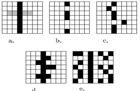
As well as the visual characteristics of color and texture, contours also have their peculiarities, to predict which detector will be the most effective [4]. In order to estimate the efficiency of the detectors, we will refer to some errors encountered when detecting contours (Perfect contour Figure 2a):
- Omission of certain pixels on the contour to be detected. It is measured by counting the number of forgotten pixels with respect to the total number of pixels of the ideal contour (Figure 2b).
- Multiple responses by detecting multiple contours. It is measured by counting the number of ambiguous pixels compared to those that are not ambiguous (Figure 2d).
- Location: this error occurs when a pixel of an unambiguous ideal outline is not in the right place. It is measured by counting the total distance between the detected contour and the ideal contour. (Figure 2c).
[image:2.612.328.558.532.682.2]- Sensitivity: This error is often related to noise and corresponds to false contours detected near the ideal contour. It is measured by counting the number of false contours and the total number of contours detected (figure 2e).
Figure 2: Examples of contour errors: a: ideal contour, b: Omission, c: relocation, d: multiple
2425
4. EDGE DETECTION PRINCIPALE
WITH GRADIENT AND LAPLACIAN
A local variation of intensity is a primary source of information in image processing. It’s measured by the gradient [4] vector function of the pixel [i, j].
4.1 The gradient in radiographic image In an orthogonal coordinate system (Oxy) where (Ox) is the horizontal axis and (Oy) the vertical axis, the image gradient (or rather the luminance f) at any point or pixel coordinates (x, y) [5] is denoted by Equation 1:
ƒ ƒ
ƒ
ƒ
The module of the gradient quantifies the importance of the contour highlighted, that is to say the magnitude of the jump intensity observed in the image:
ǁ ƒǁ
ƒ ƒ
The direction ⍺ₒ of the gradient determines the present edge in the image. Indeed, the gradient direction is orthogonal to that of the outline:
⍺ₒ arctan ƒ/ ƒ/
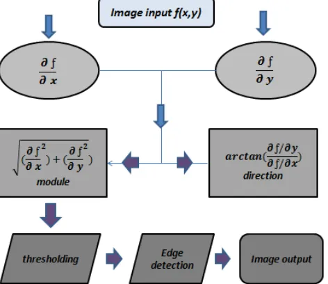
[image:3.612.73.309.515.719.2]The principle of edge detection by the use of the gradient is to calculate, in the first time, the gradient of the image in two orthogonal directions, then the gradient module. The next step is to make a selection of the most marked contours, that is to say the points of stronger contrast with adequate thresholding (Figure 3).
Figure 3: Principle of edge detection.
4.2 Gradient mask with two elements
The correlation of the mask , with a
luminance image [5] f(i, j) can be written:
, ƒ ,
0,0 ƒ , 1,0 ƒ 1,
ƒ 1, ƒ , 4
4.3 Gradient mask with three elements The gradient calculation is achieved by means of two masks, the first performing a horizontal gradient and the second performing the vertical gradient. The second mask is derived from the first by a rotation of .
[-1 0 1] and 1 0 1
Compared to the mask with two elements [6], the second mask has the advantage of producing two effects: calculating the gradient in one direction and smoothing in the other direction. This smoothing makes it a little less sensitive to noise than the previous mask.
The origin of this mask is always the central pixel. The value of the constant C can take 1 or 2 to increase the effect of smoothing.
The output pixel obtained after filtering is:
, ƒ ,
1
2 1,1 ƒ 1, 1
0,1 ƒ , 1
1
2 1,1 ƒ 1, 1
1, 1 ƒ 1, 1
1,0 ƒ 1, 1,1 ƒ 1,
1
, ƒ ,
1
2 ƒ 1, 1 ƒ , 1
ƒ 1, 1
ƒ 1, 1 ƒ 1,
ƒ 1, 1
2426 For the detection of vertical edges, other mask is used. The output pixel obtained after filtering can be put in the form:
, ƒ ,
1
2 ƒ 1, 1
ƒ 1, 1
1
2 ƒ 1,
ƒ 1,
1
2 ƒ 1,
1
ƒ 1,
1 7
Equation (7) shows the dual action: calculate on three lines the horizontal gradient then applied a vertical smoothing.
4.4 Laplacian mask with second derivative The gradient operators seen above exploit the fact that a contour in an image corresponds to the maximum of the gradient in the direction orthogonal to the contour.
However, the zero crossing of the second derivative of an intensity break also makes it possible to highlight the contour.
The second derivative is therefore determined by the Laplacian calculation:
² ƒ
²² ²²(8)
The equation can be written:
² ƒ
1,
,
,
1
,
9
Now we can define the Laplacian (Ox) by:
1, , 1,
, ,
1, (10)
1, ,
1, 1,
2 , 11 And we define the Laplacian (Oy) by:
, 1 ,
, 1 ,
,
, 1 12
, 1 , , 1
, 1
2 , (13)
So the Laplacian (Oxy) can be written:
² ƒ
1,
1,
,
1
,
1
4 , (14)
This Laplacian calculation operation can then be applied to an image via filtering with the following mask 3 * 3:
Other masks can be used for the application of the Laplacian algorithm:
After filtering the image by means of one of these filters, it is necessary to detect the zero crossings while keeping only the most marked passages. Indeed, the technique is particularly sensitive to noise due to the double derivation. It is therefore a question of not considering the noise, which can very well result in oscillations around zero, like an edge.
It is the role of the threshold S which will be used in this approach to take into account only the relatively high amplitude zero crossings corresponding to true Edge of the image.
The difference between the methods presented in this article and the classical edge detection such as Sobel, Prewitt and Robert, is that the classical masks are codes in several directions (vertical, horizontal, diagonal) and a module calculus of these directions is obligator, to have a single image that presents the edges.
The mask present in this document is applied only one liver and presents the different edge of the image.
4.5 Thresholding
The previous methods of Laplacian algorithms were used to determine the double derivation of the image that allows effectively highlighting these contours. At this level, the resulting image is expressed in gray levels, indicating here the importance of each fracture intensity.
2427 The resultant image IB (i, j) of this treatment is in black and white. White pixels (value 1) indicate the presence of an edge, the absence of black pixels (value 0).
The conversion of a gray-scale image to a black-and-white 'binarization' image after the Laplacian filter IM (i, j) image, requires the setting of the thresholding and the determining of a threshold value to represent the edges more signified and avoids the edges of the noisy.
This parameter, noted S, is chosen to present the most significant contours found from a cumulative histogram of the image at the gray level. If the value of the image pixel exceeds the threshold, the resulting pixel value is 1. Otherwise, the pixel value is set to 0:
IB (i ,j ) = 1 if IM (i ,j ) S
0 else (15)
4.6 Simulation of different operators
In this part, we present the application of different masks based on the Laplacian computation on a radiographic image, the goal is to find the mask that gives optimal results for the detection of the edges.
The comparison of these results with the methods of extraction of contours by the application of the Sobel operator, "the famous method in the field of contour detection", allows us to choose the right mask.
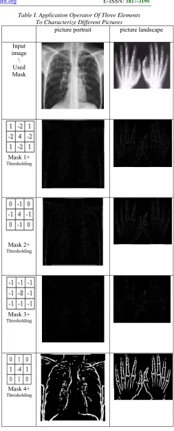
[image:5.612.303.556.77.704.2]In the first line of Table 1, we present a radiographic image of the chest of a human being (portrait image) and on the hand of a human being (landscape image), in line 2 the application of the mask [ 1 -2 1, -2 4 -2, 1 -2 1] on the two images, line 3 shows the application of the mask [0 -1 0, -1 4 -1, 0 -1] on the same images, line 4 shows the extraction of the edges by the mask [-1 -1 -1, -1 -8 -1, -1 -1 -1] and the line 5 presents the application of the mask [0 1 0, 1 -4 1, 0 1 0], and Sobel is presented in the last line.
Table I. Application Operator Of Three Elements To Characterize Different Pictures
picture portrait picture landscape
Input image
\ Used Mask
Mask 1+ Thresholding
Mask 2+ Thresholding
Mask 3+ Thresholding
2428
Mask Sobel + Thresholding
At the end, the images resulting from its different masks must be compared with the famous operator of Sobel applied on the same image in the fifteenth line. This method is based on the calculus of the concentration gradient for the extraction of edges [7,8].
We can conclude from the results below that the 3*3 element operator [0 1 0, 1 -4 1, 0 1 0] gives more accurate results, and closer to the results obtained by the Sobel operator.
The objective of these masks is the ease of implementation and the speed of processing. Their disadvantage is their sensitivity to the acoustic noise of the second derivative. However, the results are often quite broad. According to the filters of the three elements are the most used in industrial applications requiring constraints for the implementation in real time on embedded system.
5. THE NEED HARDWARE AND
SOFTWARE FOR THE PROCESSING OF RADIOGRAPHIC IMAGES IN REAL-TIME
5.1 The hardware choice for implementation To meet the needs of real time, a large number of multimedia applications and image processing, solutions for hardware implementations on reconfigurable platforms have been proposed. Most of the existing solutions are based on processing modules with 32 bits inputs / outputs. However, these solutions do not provide the memory management method for these data or are supposed to be performed by a software component.
Real-time image processing requires high computing power. For example, the standard image.jpg with a size of 640* 480 about 0.30 mega pixels per image, with an acquisition power of 100 frames per second for a CMOS camera. The size of the image may be larger [9], the amount of processing required per pixel depends on the image processing algorithm used.
The edge detection algorithm by Laplacian is a combination of two steps. The first is the product of convolution of the different pixels by the filtering mask and the second step is appropriate thresholding for the binarization of the image. Depending on the size of the masks, the processing requirements for the first convolution step can be changed. Using different algorithms with a mask size of 3 * 3 for the second derivative, both steps require more operations per pixel.
This implementation requires less complexity than the most typical 2-D convolution process due to the symmetry characteristics and separable Gaussian masks. The steps of the calculation module and the thresholding require fewer operations per pixel.
As high resolution images become more common, processing requirements will increase. High resolution images of standards typically have ten times more pixels per image. The computing load is about ten times higher. They require more DSP or a very expensive high-end DSP.
In this scenario, FPGAs provide real-time alternative image processing. FPGA effectively supports the high levels of parallel processing data flow structures "Fig. 4", which are important for the efficient implementation of image processing algorithms.
5.2The software choice for implementation In electronics, a hardware description language (HDL) is a language of a class of computer languages, specification languages, or modeling languages, for the formal description and design of electronic circuits, and more generally circuits digital logic. An HDL can describe the operation of the circuit, its design and organization; it also allows verifying its operation by means of simulation. Indeed, HDLs are text-based expression standards for describing the spatial and temporal structure and behavior of electronic systems.
Like all programming languages, the syntax and semantics of an HDL includes explicit notations to express concurrency. However, unlike most other languages, an HDL must include the explicit notion of time, which is a primary attribute for a hardware design.
2429 unique language for description, modeling, simulation, synthesis and documentation. VHDL is written independently of a particular technology or design chain, it facilitates the
passage between the different usable
technologies that evolve constantly [9,10]. The VHDL description can take one of three types of models (synthetized by Xilinx ISE software): - The behavioral model that describes the functionality of an object by a sequential algorithm or a truth table, without reference to any implementation.
- The data flow model that describes the flow between the input and the output at the bit level, by elementary equations.
- The structural model that represents the constitution of the object into a set of interconnected elementary objects (close to the schema).
6. HARDWARE IMPLEMENTATION ON
FPGA OF THE XILINX FAMILY
[image:7.612.327.567.410.626.2]For the implementation of our algorithm, we used the Xilinx Nexys-3 platform. The Nexys-3 is a complete and ready-to-use digital circuit development platform based on the Xilinx FPGA Spartan-6 LX16 (figure 4) and the VGA monitor to display the results [10,11].
Figure 4: Nexys-3 Card Architecture [10]
Nexys-3 with The Spartan-6 is optimized for high-performance logic and offers more than 50% higher capacity, more performance and
more resources compared to the Nexys2 Spartan-3 500E FPGA.
The Spartan-6 LX16 features include:
- 2,278 slices each containing four 6-input LUTs and eight flip-flops
- 576Kbits of fast block RAM
- 2 clock tiles (four DCMs and two PLLs) - 32 DSP slices
- 500 MHz + clock speed Preview on Spartan-6 circuit
In addition to the Spartan-6 FPGA, the Nexys-3 offers an enhanced collection of peripherals, including Micron's 32-bit Phase Change non-volatile memory, 10/100 Ethernet, 16 MB of cellular RAM, USB UART, a USB host port for mice and keyboards, and an enhanced high-speed expansion connector.
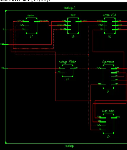
The algorithm was developed on Xilinx ISE interface and all the blocks are programmed in VHDL with the following block diagram (Figure: 9):
Our project consists of several blocks, which are other than VHDL programs:
[image:7.612.92.308.434.666.2]6.1 Block program "Memory Playback" Since the image is not necessarily the same size as the screen, the program is necessary for the correct positioning of the image on the screen (Figure 5).
Figure 5: Block memory generator for Xilinx Spartan-6
6.2 Block program "Synchronization"
2430 the entire screen. By manipulating these signals, the images are formed on the monitor screen [12].
Figure 6: H and V synchronization
6.3 Block program "Memory"
The "Memory" block that exists in the party IP (intellectual property) to the Xilinx software is configured according to the size of the image that will store.
Each memory cell contains 8 bits (8 bits is the value which is coded each RGB pixel).
The DDR2-Micron memory, used in the Xilinx platforms, is organized into 4 data banks addressed by the two address lines (BA0, BA1), each Bank is organized into a matrix of cells (2 ^ 13 lines × 2 ^ 10 columns), each cell is composed of 64bits.
The lines are addressed by A0-A12 and the columns are addressed by the same lines A0-A9, thus the need to use a multiplexer at the DDR2 controller [13].
If you only manipulate the luminance signal (on 8 bits), each memory cell in the DDR2 can contain 8 pixels. Similarly, a line of memory can contain 8 × 2 ^ 10 pixels, and a 256 × 256 pixels image occupies 8 lines of memories [54]. From this architecture, we notice that the DDR2 promotes the reading of packet data and even several packets at the same time.
The logical user communicates with the memory controller via a FIFO based on a user interface. This interface consists of three related buses: - A control bus / FIFO address, this bus accepts Read / Write commands and the corresponding memory address;
- A FIFO type Write data bus that accepts writing data when a write command is sent on the control bus;
- A FIFO type read bus, on which data is read with a Read enable command, to the processing blocks.
6.4 Block program "VGA Screen"
The program's role to define the VGA monitor is controlled by five 10-bit coded signals: red (3 bits), green (3 bits), blue (2 bits), horizontal sync and vertical sync (2 bit).
The three color signals, collectively known as the RGB signal are used to control the color of a pixel at a location on the screen (figure 7). In order to produce other colors, each color analog signal is to be supplied with a voltage between 0.7 and 1.0 volts for varying the intensities of the colors.
Figure 7: VGA screen
6.5 Block program "algorithm"
[image:8.612.335.573.378.569.2]2431 Figure 8: Processing of data streams in parallel
FIFOs are implemented using multiple integrated M4K memory blocks, which are a size of 4 kbps each. The image of the edge detection result is stored in the blocks of RAM built in the Spartan-6 [14] device. These large blocks of integrated RAM can be used to store temporarily the edge image when 2 bits are allocated to each pixel location.
[image:9.612.314.574.196.605.2]Figure 9 shows a diagram of the different blocks programmed in VHDL and synthetized by Xilinx ISE software [10,11].
Figure 9: The blocks implemented on Xilinx ISE
In table 2 we present some statistics generated by
the software ISE-XILINX during the
implementation of our programs on the FPGA Spartan-6.
Flip Flop pair for this architecture represents one LUT paired with one Flip Flop within a slice. A control set is a unique combination of clock (reset, set, and enable) signals for a registered element. The Slice Logic Distribution report is not meaningful if the design is over-mapped for a non-slice resource or if Placement fails.
Table Ii. Device Utilization Summary
Slice logic utilization Used Available Utilization
Number of slice Registers 63 18224 01%
Number of slice LUTs 95 9112 01%
Number used as Memory 00 2176 0%
Number Used as logic 94 9112 01%
Number of occupied slices 32 2278 01%
Number MUX cys used 40 4556 01%
Number with an unused Flip Flop
36 98 36%
Number with an unused LUT 03 98 03%
Number of fully used LUT-FF
pairs 59 98 60%
Number of slice register sites lost to control set restrictions
25 18224 01%
Number of bonded IOBs 20 232 08%
Number of LOCed IOBs 12 20 60%
Number of RAM B16BWERs 20 32 62%
Number of RAM B8BWERs 00 64 00%
Number of BUFIO2/ BUFIO2-2CLKs
00 32 00%
Number of BUFIO2FB/
BUFIO2FB-2CLKs 00 32 00%
Number of BUFG/
BUFG-MUXs 02 16 12%
FPGA components allow you to implement two types of SoPCs. The first type of SoPC uses only soft IP processors such as MicroBlaze. The number of integrated processors on the same component depends on the resources of the component used.
[image:9.612.92.306.401.653.2]2432 Xilinx) by following the steps presented in Figure 10.
Figure 10 : Flot de conception Xilinx [6].
7. RESULTS OF IMPLEMENTATION
AND DISCUSSION
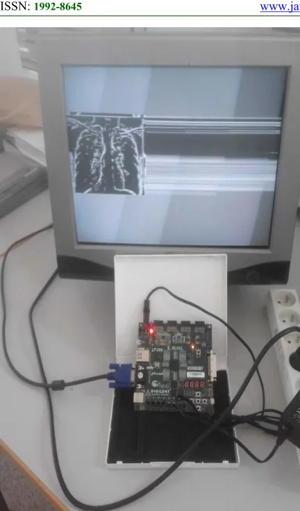
To display the processed images we used a VGA screen connected directly to a Xilinx Spartan-6 FPGA circuit. Figure 11 shows the pre-processing image and Figure 12 shows the same image after processing.
We used a radiographic image with a resolution of 200x200. The module is fully pipelined where a resulting pixel is calculated at each clock cycle. With this rate and the clock frequency, it is possible to treat more than 400 image frames per second at 200x200 resolutions.
In addition, the entire chain has been developed
following the appropriate methodology,
Algorithm Architecture. With the regular calculations, the necessary reduced memories and the important intrinsic parallelism, it forms an ideal candidate for hardware implementation on embedded systems [13-14].
In terms of performance and power consumption, FPGAs are commonly the lowest in embedded systems, and can compete by being available quickly, reprogrammable and manufactured with the latest technology. They provide an attractive alternative when the resources (cost, time) required by ASIC development are not available. The ability to parallelize operations and perform customizable functions also makes them competitive with the sequential microprocessor [15].
[image:10.612.92.289.98.286.2]2433 Figure 12: The Image Results After Treatment.
The design is scalable to handle high-resolution images while keeping the clock rate at 100MHz. Our solution is capable of processing a standard images tram up to 25 frames per second, as well as X-ray image acquisition equipment at high speed, which require more than 30 frames per second.
It is possible to increase the frequency above 100 MHz by introducing more pipeline stages at the expense of increased resource utilization [16-17]. But the uses of high resolution images require a more powerful processor that exceeds the range Spartan, in talking about the Virtex range, high performance at frequencies exceeding 500MHz. To increase the storage capacity on the Spartan-6 circuit, three external memories available on the Xilinx Nexys-3 platform can be configured: a 128 Mbit cellular RAM (pseudo-static DRAM), a parallel non-volatile PCM 128Mbit (memory of phase change); and a 128Mbit PC serial device. To access these external memories, whatever the type, a memory controller is used which serves
as an intermediary between the user program and the physical memory. The controller is also used to perform the operations of commands; physical address calculations from logical addresses, data logging and addresses in FIFOs for Read / Write, automatic refresh [18-19]. The user program deals only with the logical address generation part as well as the Read / Write commands.
8. CONCLUSION
In this work, we propose an implementation of edge detection by Laplacian algorithms on an FPGA. The presented method is based on the detection of the zeros in the change of the intensity, the masks of convolutions obtained by the calculus of the second derivative (for variation of the intensity) and a thresholding to select the contours the strongest in the radiographic image.
The results obtained show the clear presence of all the edges that exist in the images, these results can be used as a diagnostic tool to differentiate the zones of the image in order to characterize the fractures and to extract reduced information, often relevant to characterize the images acquired by X-ray equipment.
The use of a Spartan-6 FPGA circuit demonstrates its ability to handle high resolution VGA images, while maintaining the clock frequency used (100 MHz) to process images of high resolution X-ray equipment (25 frames per second), as well as applications based on computer vision.
In this context, the Field Programmable Gate Array (FPGA) with its large integration and reconfiguration capabilities make it a key component for rapidly developing prototypes. In order to encourage the widespread diffusion of such circuits, it is necessary to improve the development environments to make them more accessible to non-experts in electronics.
REFERENCES:
[1]. D. Marimont, Y. Rubner, "A probabilistic Frameword for Edge Detection and selection of Scale", Proceedings of the International Conference of the IEEE Computer Vision, 207-214, January 1998. [2]. T. Lindeberg, "Edge Detection and Ridge
2434 International Journal of Computer Vision, Vol. 30, No. 2, 117-154, 1998.
[3]. D. Maar, E. Hildreth, "Theory of edge
detection," Proceedings Royal Soc.
London, vol. 207, 187-217, 1980.
[4]. Yitzhak Yitzhaky et Eli Peli – “A Method
for Objective Edge Detection Evaluation and Detector Parameter Selection” – IEEE transactions on pattern analysis ans machine intelligence, vol. 25 No 8 - Août 2003
[5]. J. Malik, S. Belongie, T. Leung and J. Shi,
Contour and texture analysis for image segmentation”, IJCV, vol.43, no.1,2001.
[6]. Duncan D-Y Po and Minh N. Do. - «
Directionnelmultiscale modeling of images using the contourlet » - Coordinated Science Lab and Beckman Institute, University of Illinois at Urbana-Champaign - Urbana IL 61801 , 2003
[7]. J.F. Canny, "A computation approach to edge detection," IEEE Transactions on Pattern Analysis and Machine Intelligence, vol. 8, 6pp. 769-798, November 1986. [8]. M. N. Do et M. Vetterli, “The contourlet
transform: an efficient directional
multiresolution image representation”. IEEE Transactions Image Processing, 2003.
[9]. W. He and K. Yuan, "An improved Canny
Edge Detector and its Realization on FPGA," Proc. of 7ili World Conference on Intelligent Control and Automation, 2008.
[10].
http://www.xilinx.com/products/design-tools/ise-design-suite.html [11].
http://store.digilentinc.com/fpga-programmable-log
[12].R. Wang, G. Cohen, K. M. Stiefel, T. J. Hamilton, J. Tapson, and A. van Schaik,
An FPGA Implementation of a
Polychronous Spiking Neural Network with Delay Adaptation. frontiers in Neuroscience, 2013.
[13].I. Bouganssa, M. Sbihi and M. Zaim
"Implementation of Edge Detection Digital Image Algorithm on a FPGA" MATEC Web of Conferences. Vol. 75, No 03003 Sept 2016
[14].I. Bouganssa, M. Sbihi and M. Zaim
“Implementation on a FPGA of Edge Detection Algorithm in Medical Image and
Tumors Characterization” DOI:
10.1109/ICMCS.2016. 7905655. IEEE. 2016.
[15].I. Bouganssa, M. Sbihi and M. Zaim
“Implementation in an FPGA circuit of Edge detection algorithm based on the Discrete Wavelet Transforms” Journal of Physics: Conf. Series Vol. 870 No 012016 (2017)
[16].Xilinx Inc., ‘Xilinx Memory Interface Generator (MIG) User Guide, DDR SDRAM, DDRII SRAM, DDR2 SDRAM and RLDRAM II Interfaces’, Document: UG086 (v2.0), 2007.
[17].S. Nazari, M. Amiri, K. Faez, and M.
Amiri, Multiplier-less digital
implementation of neuron–astrocyte
signalling on FPGA. Neurocomputing, 2015.
[18].Duncan D-Y Po and Minh N. Do. - «
Directionnel multiscale modeling of images using the contourlet » - Coordinated Science Lab and Beckman Institute, University of Illinois at Urbana-Champaign - Urbana IL 61801 , 2003
[19].Michal Strzelecki, PrzemyslawBrylski, H. Kim ‘FPGA-Based System for Fast Image Segmentation Inspired by the Network of Synchronized Oscillators’ International Conference on Artificial Intelligence and Soft Computing pp 580-590, ICAISC 2017.