BIROn - Birkbeck Institutional Research Online
Catao, L.A.V. and Fostel, A. and Kapur, Sandeep (2009) Persistent gaps and
default traps. Journal of Development Economics 89 (2), pp. 271-284. ISSN
0304-3878.
Downloaded from:
Usage Guidelines:
Please refer to usage guidelines at or alternatively
BIROn -
B
irkbeck
I
nstitutional
R
esearch
On
line
Enabling open access to Birkbeck’s published research output
Persistent gaps and default traps
Journal Article
http://eprints.bbk.ac.uk/1959
Version: Pre-print (Working Paper)
Citation:
© 2009 Elsevier
Publisher version available at:
http://dx.doi.org/10.1016/j.jdeveco.2008.06.013
______________________________________________________________
All articles available through Birkbeck ePrints are protected by intellectual property law, including copyright law. Any use made of the contents should comply with the relevant law.
______________________________________________________________
Deposit Guide
Birkbeck ePrints
Birkbeck ePrints
ISSN 1745-8587
Birkbeck Workin
g
Pa
p
ers in Economics & Finance
School of Economics, Mathematics and Statistics
BWPEF 0803
Persistent Gaps and Default Traps
Luis A V Catão
IADB and IMF
Ana Fostel
George Washington University
Sandeep Kapur
Birkbeck, University of London
Persistent Gaps and Default Traps
∗
Luis A. V. Cat˜
ao
†Ana Fostel
‡Sandeep Kapur
§February 2008
Abstract
We show how vicious circles in countries’ credit histories arise in a model where output persistence is coupled with asymmetric infor-mation between borrowers and lenders about the nature of output shocks. In such an environment, default creates a pessimistic outlook about the borrower’s output path. This translates into higher debt-to-expected-output ratios, pushing up interest rates and hence debt servicing costs. By raising the cost of future repayments, this creates “default traps”. We provide empirical support for the model by build-ing a long and broad cross-country dataset spannbuild-ing over a century. This data is used to provide evidence on the existence of a history-dependent “default premium” and to show that the effect of output persistence on sovereign creditworthiness is significant and consistent with the model’s predictions after controlling for other determinants of sovereign risk.
JEL Classification: F34, G15, H63, N20.
Keywords: Sovereign default, spreads, persistence
∗We thank Marcos Chamon, Roberto Chang, John Driffill, Eduardo Fernandez-Arias,
Gordon Hanson, Alejandro Izquierdo, Graciela Kaminsky, Enrique Mendoza, Andrew Pow-ell, Ron Smith, Carlos Vegh, Vivian Yue as well as seminar participants at GWU, IADB, IMF, NBER, University of Maryland, University of Warwick, and the World Bank for comments on earlier versions of this paper. The usual caveat applies.
†IADB and IMF. The views expressed in this paper are the authors’ alone and do not
necessarily reflect those of the IADB or IMF.
‡George Washington University, Washington, DC.
1
Introduction
A major stylized fact about the history of sovereign borrowing is the per-vasiveness of serial default. Lindert and Morton (1989) find that countries that defaulted over the 1820-1929 period were, on average, 69 percent more likely to default in the 1930s, and that those that incurred arrears and con-cessionary schedulings during 1940-79 were 70 percent more likely to default in the 1980s – clearly suggestive of substantial persistence in creditworthiness patterns. While these probability estimates are not conditioned on countries’ fundamentals, evidence provided in Rogoff, Reinhart, and Savastano (2003) indicates that serial default is only loosely related to countries’ indebtedness levels and other fundamentals. They show that serial defaulters have lower credit ratings and face higher spreads at relatively low indebtedness levels – a phenomenon they call debt intolerance. The experience of such debt-intolerant countries – involving a vicious circle of borrowing, defaulting and being penalized with higher interest rates – stands in sharp contrast with that of countries that manage to undergo a virtuous circle of borrowing and repayment with declining sovereign spreads.
An associated empirical regularity is that default rarely entails complete exclusion from international capital markets but mainly a re-pricing of coun-try risk (higher spreads), at least for some time. This regularity is at odds with much of the theoretical literature: in early models (notably Eaton and Gersovitz, 1981) it is the threat of permanent exclusion from capital mar-kets which is crucial to sustain sovereign lending; later models allowed for this exclusion to be temporary but with random re-entry rules which are not price-dependent (Aguiar and Gopinath, 2006; Arellano, 2006).1 In
prac-tice, default is often punished not through outright denial of credit or fixed re-entry rules but a worsening of the terms on which the country can bor-row again.2 Provided that borrowing needs are not too price elastic, the
1A notable exception is Eaton (1996), who constructs a model where an endogenous
bond re-pricing creates a deterrent mechanism. Earlier studies have also well acknowledged the problems associated with the assumption of strict market exclusion, including that of coordination problems among multiple lenders (Kletzer, 1984), and borrowers’ retained ability to invest in risk-free international assets after default, which would render default-free lending unsustainable without other penalties (Bulow and Rogoff, 1989).
2In fact, not only is permanent exclusion quite rare, but even temporary loss of market
sovereign will continue to tap the market – absolute exclusion representing only the limiting case in which lenders’ enforcement technology is so weak that country spreads may become prohibitively large for any borrowing to take place.
This paper argues that two structural features that are typically found in emerging markets help explain both stylized facts. These structural features are that output shocks are not only typically large, thus producing high cyclical variability about trend growth, but also highly persistent.
That output volatility is generally high among emerging markets is a well-documented phenomenon (see, for instance, Kose et al., 2006). Recent work has related such volatility to a number of long-lasting structural features. These range from domestic institutions (Acemoglu et al., 2005), commod-ity specialization (Blattman et al., 2007) to imperfections in international capital markets that limit these countries’ ability to issue domestic-currency denominated sovereign debt, thus rendering them more vulnerable to cur-rency fluctuations (Eichengreen et al., 2003).
What has received less attention in the literature, however, is the fact that output volatility is often coupled with considerable persistence of out-put shocks. For a given dispersion of shocks (conditional outout-put volatility), higher persistence implies that associated output fluctuations will be larger.3 So the same unconditional output volatility may be generated by different combinations of persistence and dispersion of shocks. Yet, as we show be-low, it is important to disentangle the effects of these distinct parameters on sovereign risk. On a broader analytical level, such a separation is impor-tant as well because there are distinct macroeconomic mechanisms behind shock persistence in emerging-market economies. These include the presence of short-run supply-side inelasticities that make primary commodity price
While there is some debate about whether recalcitrant borrowers are consistently punished with higher spreads (Eichengreen and Portes, 1986; Ozler, 1993), broader historical data that we present in this paper indicates that bond yields typically do rise in the wake default events and remain higher than average (albeit declining) for several years after those events. This is also consistent with evidence provided in Flandreau and Zumer (2004) on the behavior of spreads during the pre-WWI period.
3To see this, let y
i,t =ρyi,t−1+ωi,t where yi,t is output of countryi in period t, ρis
the persistent parameter and ω is an i.i.d shock. Then we have that the unconditional output volatility isσyi,t=
σωi,t
√
shocks long-lasting,4 the various frictions (political as well as economic) which
make fiscal policy more procyclical in these countries5, as well as financial and institutional frictions that typically magnify the sensitivity of domestic credit to loan collateral values and balance sheet mismatches; as the latter can induce prolonged spirals of output contraction or expansion, including painful episodes of debt deflation (see, e.g., Calvo, 1998; Mendoza, 2006), they tend to exacerbate overall output persistence.
[Tables 1 and 2 here]
This begs the question as to whether, and to which extent, output has in-deed been typically more volatile and persistent among defaulters and serial defaulters. Tables 1 and 2 provide suggestive evidence. Using data spanning the century-and-quarter period from dawn of international bond financing in the 1870s through 2004, the tables report the standard deviation as well as the first autoregressive coefficient of HP-filter de-trended output for each country over the three main sub-periods delimited by the World Wars. As is immediately apparent from group medians, defaulting countries typically display higher volatility and persistence than non-defaulting countries on av-erage. Further, these cross-country differences appear to be typically even higher between serial defaulters and non-defaulters, and are consistently ob-served for certain countries over the entire 1870-2004 period. The postulated relationship also appears to be robust to potential reverse causality emanat-ing from the effects of defaults on the volatility and persistence of output
4See Cashin et al. (2000) and references therein for empirical evidence on the
persis-tence of commodity price shocks. Mendoza (1995) finds that terms of trade variations typically account for up to one-half of business cycle fluctuations in developing countries.
5In a recession, a contractionary fiscal stance tends to delay recovery, which
shocks: when we eliminate from the sample all default events and their im-mediate aftermaths, defaulters continue to display greater output volatility and shock persistence relative to their more virtuous peers.
Against this background, the aim of this paper is twofold. The first is to lay out a model that shows how, in the presence of informational asymme-try, the combined effects of volatility and persistence of output shocks can generate some path dependence in countries’ credit history. In particular, when borrowers are better informed than lenders about the persistence of their output shocks, repayment choice – default vs. repayment – can trig-ger a discrete shift in expectations about the borrower’s future output path: upon observing default, lenders might end up “assuming the worst” about the repayment prospects on future loans. If so, fresh lending is likely to be at significant higher interest rates. In contrast, repayment of past loans creates a more favorable outlook for future repayment and justifies future lending at lower interest rates. The difference between interest rates that the sovereign borrower faces after default relative to those following repayment can be viewed as a default premium. Ex-ante such a default premium constitutes a deterrent mechanism that induces countries to pay even in the absence of output penalties featuring elsewhere (e.g., Sachs and Cohen, 1985; Obstfeld and Rogoff, 1996; Alfaro and Kanczuk, 2005). Ex-post, such a default pre-mium raises the cost of future repayments beyond what is justified by other fundamentals (including past history of output volatility and persistence), and thus exacerbates the likelihood of future defaults. We use the notion of
default traps to capture the idea that, in the presence of fragile expectations, the impact of a negative output shock on country risk can be amplified and throw an otherwise solvent country on the path of serial default. More pre-cisely, a country can fall into a default trap in that, once it defaults, it is more likely to default again in the future, compared to another country with identical fundamentals.
historical levels – to 2004. This database is not only longer than previous historical studies on sovereign risk (e.g. Obstfeld and Taylor, 2003) but also has better output data for some countries and encompasses a wider set of variables (See Appendix 2). Our results clearly indicate that countries with more volatile and persistent output shocks are likely to face higher ex-ante interest spreads and thus more likely to be caught into default traps. Con-sistent with our theoretical results, we also find evidence of a significantly positive default premium and of such a premium being rising with the un-derlying persistence of deviations between actual and expected output - the so-called output gap. This offers one explanation for why country spreads (measured relative to the risk-free interest rate) react strongly to default an-nouncements even after controlling for changes in other fundamentals. Such a significant and typically long-lasting rise in spreads in turn makes countries more likely to fall prey to default traps.
Other papers have explored the implications of informational asymme-tries in models of sovereign debt.6 Typically, in these papers, observed de-fault provides a signal about some unobservable borrower characteristic that is relevant to the lender’s payoff. For instance, if borrowers differ unobserv-ably in their discount rates, default may reveal the borrower to be relatively short-termist. However, these models do not fully develop the implications of these signals on price of future debt, so effectively overlook the default pre-mium mechanism outlined in this paper. Eaton (1996) is notable exception: he develops a model in which sovereign borrowers differ in the vulnerability to the enforcement technology, rendering one less likely to default than the other, and this does affect the price of future debt. However, to the extent that the asymmetry of information in our paper relates to the borrower’s out-put process, it allows us to examine directly the effects of outout-put persistence on country risk, allowing us to discuss the possibility of default traps.
The plan of the paper is as follows. Section 2 lays out the model, our main theoretical results and discusses their robustness. Section 3 reports the econometric results. The paper concludes with a summary of the main find-ings and a brief discussion of the policy implications in Section 4. Appendix 1 presents proofs of the theoretical propositions while Appendix 2 describes the data.
2
Model
2.1
The Sovereign Borrower
A sovereign borrower issues bonds in international capital markets to finance investment in one-period projects. We develop our model in a simple setting that involves three periods, t= 0,1, and 2. The sovereign invests in periods 0 and 1. Investment It at t = 0,1 returns expected output ¯Yt = f(It) in
period t+ 1, where f is concave. The country’s actual output is stochastic due to two sources of output uncertainty: a persistent shock and a transient shock. Specifically, output at t= 1,2 is given by:
˜
Y1 =f(I0) + ˜1+ ˜ω1 (1)
6See, for instance, Kletzer (1984), Atkeson (1991), Calvo and Mendoza (2000), Alfaro
˜
Y2 =f(I1) +ρ˜1+ ˜ω2 (2)
Here random variable 1 is a persistent shock, with mean 0 and standard
deviation σ. Let Φ() denote the distribution of persistent shocks and φ()
the associated density function. The parameter ρ ∈ (0,1) measures the persistence of the shock from period 1 to period 2. Random variables ωt
denote transient shocks: these are independent with mean 0 and standard deviation σω.7
For tractability we begin by assuming that investment levels I0 and I1
are exogenously given. This allows us to focus on the central concern in our model: the sovereign borrower’s repayment decisions in periods 1 and 2, for bonds issued in the previous periods. As the assumption may seem strong, we later provide theoretical justification for it and examine the implications of relaxing it.
The sovereign’s utility function is linear in payoffs. When making its period-1 repayment choice, the sovereign maximizes E( ˜y1 +βy˜2), where ˜yt
denote its output net of any repayments andβ ≤1 is a discount factor. With this linear specification, the sovereign cares only about expected future payoff associated with its current choices, an assumption that makes the analysis tractable.
Investment is entirely financed by borrowing. To fund its investment requirement It at t, the sovereign must issue one-period bonds of face value
Dt+1, where
ptDt+1 =It, (3)
and pt denotes the issue price of bonds.
2.2
Bond Markets and Sovereign Spreads
The bond market is competitive, with risk-neutral lenders who are willing to subscribe to bonds at a price that allows them to break-even. The issue price of bonds, determined endogenously in the model, depends on the perceived likelihood of default. We assume that in the event of default, bondholders
7The shock variances are such that ¯Y
t <˜t+ ˜ωt is a negligible probability event, so
can enforce partial recovery obtaining a proportion c < 1 of the face value of outstanding debt. If the sovereign is expected to default at t + 1 with probability πt+1, the expected return to a bond of unit face value is πt+1c+
(1−πt+1). A risk-neutral lender who acquires a unit bond at priceptat time
t expects to break even in period t+ 1 if
[πt+1c+ (1−πt+1)] =ptRf, (4)
where Rf = 1 +rf is the exogenously-given gross risk-free interest rate. The
competitive market-clearing price of bonds is
pt=
1−πt+1(1−c)
Rf
. (5)
As pt ∈ [c/Rf,1/Rf], the bond price is positive as long as c > 0. The price
of bonds pt(πt+1) is decreasing in the anticipated probability of default.8
Bond yields, as conventionally defined,
it=
Rf
1−πt+1(1−c)
−1 (6)
are increasing in the probability of default, as is the sovereign spread over the risk-free rate of interest, which equals (it−rf).
2.3
Asymmetric Information and Default Premium
We assume that while ¯Yt, ρ, and the distribution of shocks are common
knowl-edge, only the sovereign borrower observes the magnitude of its period-1 shocks directly. Bondholders do not, but make an inference about its likely realization by observing the sovereign’s repayment decision in period 1. The updated beliefs are used to form expectations of future output, and hence the probability of future default.
In order to show how this information structure gives rise to the existence of a default premium, we provide an informal discussion of the sequence of
8Eaton and Gersovitz (1995) provide an interesting argument as to why the probability
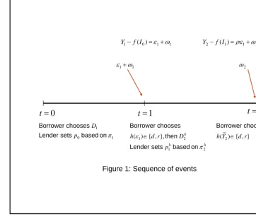
events and equilibrium before we state our formal result in the next sub-section. At time t= 0, the sovereign issues one-period bonds with face value
D1to meet its initial investment requirementI0, so thatp0D1 =I0. The issue
pricep0 of these bonds is determined endogenously, based on expected default
risk. At time t = 1, the sovereign observes its output shock and chooses between default, d, or repayment, r. The period-1 repayment “history” is denoted by h∈ {d, r}.
On observing the sovereign’s repayment history in period 1 bondholders update their beliefs in accordance with Bayes’ rule. The repayment decision affects bondholders’ beliefs about the sovereign’s future output and, hence, the probability of future default denoted as πh2, varies with history h. The sovereign then issues new bonds at t = 1, at priceph1 ≡p1(πh2) to finance its
period-1 investment requirement I1. It requires
ph1D2h =I1. (7)
Given the fixed investment requirement I1, if the issue price depends on h,
so does the required nominal bond issue, Dh
2.
Finally, at t = 2 the sovereign chooses whether or not to repay its debt obligationDh
2. Given our choice of a finite-horizon framework, partial capture
provides insufficient deterrence against default in the final period. In the absence of other penalties, att = 2 the sovereign will default with probability one. To avoid the trivialities associated with this case, we assume that default in the final period is also punished with sanctions that cause the sovereign to lose a fraction s of its current output ˜Y2.9 Figure 1 depicts the sequence
of events.
[Figure 1 here]
Our analysis begins, as is standard, from the final period. Given the enforcement technology, repayment will be rational in the final period if and only if the cost of sanctions exceeds any direct gain from reneging on
9As in Sachs and Cohen (1985) and Obstfeld and Rogoff (1996) we assume that
repayments. We show that the borrower repays at t = 2 if and only if the debt-to-output ratio exceeds a critical threshold.
The borrower’s repayment choice in period 1 depends on a comparison of the benefit and cost of default. Default has benefits in terms of repay-ments avoided (except some which is captured). Default is costly because to the extent it alters market perceptions of future default risk, the cost of financing fresh investment rises. Given this trade-off, we show formally that the optimal repayment rule in period 1 also satisfies a threshold property: the borrower will repay in at t = 1 if and only if the realization 1 of the
persistent shock is above some threshold, e1. The equilibrium value of this
threshold will be denoted as e∗1.
The informational asymmetry between the borrower and bondholders translates into differences in beliefs about the sovereign’s second-period out-put. The sovereign, who observes the realization of the persistent shock 1,
expects ˜Y2 to be distributed with mean f(I1) +ρ1 and standard deviation
σω. Let the associated (cumulative) distribution function beF|1( ˜Y2).
Bond-holders, on the other hand, do not observe 1 but only the repayment history
h. Let Gh( ˜Y2|e1) denote the lenders’ distribution over ˜Y2 if they observe
his-tory h and if they believe the borrower’s repayment threshold to bee1. The
distributions F|1 and Gh summarize the information asymmetry. Together
{e1,Φ, F|1, Gh} denote the evolution of beliefs over time.
In this setting, default in period 1 signals the realization of an adverse output shock and, given persistence, creates a pessimistic outlook regarding the sovereign’s future output and default risk. On the other hand, repayment generates a more favorable outlook. This translates into higher conditional probability of future default: that is, we have πd2 > πr2. Using equation (5), this implies thatpr
1 (the issue price of new bonds contingent on repayment at
t = 1) exceedspd
1(the corresponding value contingent on default). Expressing
the same idea in term of bond yields, a country with a history of default is required to offer higher bond yields id
1 to attract funds than it would have
had to pay with a sound repayment history, ir
1.
We refer to the differenceid1−ir1 (or equivalently, the difference in prices
pr
1 −pd1) as the default premium. Note that this default premium is purely
of a positive default premium is a key feature of our model. This feature is formally shown in the equilibrium described below.
2.4
Default Traps Equilibrium
We model the interaction between the borrower and lenders as a game. For descriptive purposes, it is convenient to consider the mass of lenders as a single player: this ‘lender’ sets the bond price so that the expected return on bonds equals the opportunity cost of capital. Thus the lender’s strategy is given by prices (p0, pr1, pd1) that allow it to break even, given the perceived
likelihood of default (π1, πr2, πd2).
A strategy for the sovereign borrower involves the following elements: bond issuance D1 att = 0, repayment choice h∈ {r, d} followed by
history-contingent bond issuance Dh
2 at t = 1, and, finally, the repayment choice at
t = 2.
Beliefs in the game are specified by the critical thresholde1 which
deter-mines the the borrower’s repayment choice in period 1, the prior distribution Φ of persistent shocks, and the posterior distributions F|1 and Gh over the
final period output.
We consider a Perfect Bayesian Equilibrium (PBE) of this game, at which players choose strategies that are optimal given their beliefs and other player’s strategies, and beliefs are consistent with strategies and observed actions. Proposition 1 describes such an equilibrium.
Proposition 1 There exists an e∗1 such that the following is a PBE of the game:
1. The borrower’s repayment decision at t= 1 is given by
h(1) =
(
r if 1 ≥e∗1
d if 1 < e∗1
The borrower repays at t= 2 if and only if Y˜2 ≥[(1−c)/s]Dh2.
2. The lender’s strategy is given by (p0, pr1, pd1)at which it breaks even each
3. The lender’s beliefs in period 0 are given by the prior distributionΦ(1).
At t = 1, if it observes default, beliefs are given by the density function
γd(1|e∗1) =
( φ(1)
Φ(e∗1) if 1 < e ∗ 1
0 otherwise
If, instead, the lender observes repayment
γr(1|e∗1) =
( φ(1)
1−Φ(e∗
1) if 1 ≥e ∗ 1
0 otherwise.
The proof of this Proposition is provided in Appendix 1, but we high-light two key features of the equilibrium. First, the equilibrium suggests the possibility of what we refer to as default traps. Second, the positive default premium constitutes an endogenous deterrence mechanism that can support repayment of debt even in the absence of other penalties.
Given the information asymmetry, the borrower’s period-1 choice – de-fault vs. repayment – can be quite informative. Dede-fault triggers a discrete shift in expectations as the lender infers that the realization of the persistent shock1 must lie below the criticale∗1, that is, in the lower tail of distribution
Φ. In effect, the lender ‘assumes the worst’ about the future output path of a borrower who defaults. Such pessimism, combined with the lender’s need to break-even, implies that fresh borrowing is sustainable only at significantly higher spreads, or equivalently, lower bond prices. If, as in our model, the investment requirement is relatively inelastic, the required volume of issued debt needs to be even higher to compensate for low issue prices. This, in turn, raises the risk of future default. In contrast, a good credit history cre-ates a more favorable outlook, with higher bond prices, lower nominal debt requirements and significantly lower risk of future default.
country risk can be amplified and throw an otherwise solvent country on the path of serial default. More precisely, a country can fall into a default trap in that, once it defaults, it is more likely to default again in the future, compared to another country with identical fundamentals. The underlying mechanism is entirely symmetric, with a good repayment history creating a virtuous cy-cle of lower spreads, smaller borrowing requirements and significantly lower risk of default.
2.5
Comparative Statics
The deterrence mechanism allows us to explore how the equilibrium varies with the degree of persistence. To appreciate this mechanism, note that beliefs must be such that the borrower is just indifferent between default and repayment at the threshold e∗1. The gain from repayment comes from the more favorable terms of access to future borrowing. Let Vr
2 denote the
continuation payoff for the borrower following repayment andV2dbe the con-tinuation payoff following default. These concon-tinuation values depend on 1
(as it conditions the borrower’s beliefs F|1 about future output), and on
expectations e1 regarding the repayment threshold (as that conditions the
lender’s posterior beliefs). The difference Vr
2 −V2d captures the anticipated
future gain from repayment relative to default. The direct cost of repayment is given by (1−c)D1. Given the prior distribution Φ(1), the ex-ante
likeli-hood of default at t = 1 equals Φ(e1). Recall that for risk-neutral lenders to
break even we must have
[1−(1−c)Φ(e1)]D1 =RfI0. (8)
Figure 2 captures the trade-off between the cost and benefit of repayment. The upward-sloping curve represents the direct cost of repayment, CR(e1)≡
(1−c)D1(e1), as function of e1. As the solution D1(e1) to (8) is increasing
in e1, so is CR(e1). The downward-sloping curve represents the discounted
value of the future benefit from repayment,BR(e1)≡β[V2r−V2d]. The proof
of Proposition 1 shows thatBR(e1) is decreasing in the repayment threshold
e1.10 At the equilibrium, the value ofe1must be such thatBR(e∗1) =CR(e ∗ 1).
10The proof also shows thatBR is increasing in the realization of the shock
1, so that
the borrower is more likely to repay when output is high. This is not inconsistent with the feature that the gain from repayment is decreasing in the repayment thresholde1, which
[Figure 2 here]
Both benefit and costs vary with the other parameters of the model, so variations in these will affect the equilibrium. Proposition 2 examines the impact of changes in the persistence parameter ρ.
Proposition 2 An increase in the persistence parameter ρ raises the equi-librium default premium and the ex-ante probability of default in period 1.
Once again, Appendix 1 provides a formal proof but the intuition is sim-ple. Greater persistence implies that future output shocks are more closely related to period 1 shock 1, so that the informational value of observed
de-fault is greater. The future gain from repayment relative to dede-fault would be larger for any given repayment threshold e1, or in term of our graphical
representation, the downward sloping curve must be higher everywhere for a larger persistence parameter. At e∗1, the gain from repayment now exceeds the gain from default. To restore the balance between the gain from repay-ment and default, equilibrium beliefs regarding the threshold needs to adjust to a new, higher value (call it e∗∗1 ). This implies a higher ex-ante probability of default and, by the break-even condition, higher sovereign spread att = 0. To put it differently, the strength of the deterrence mechanism determines the riskiness of the loans that can be made. Stronger deterrence can support debt contracts with larger nominal value, which in our setting tend to be associated with greater probability of default.
Clearly, for persistence to play such a role in exacerbating the default trap mechanism, volatility of output shocks must be relatively large. As discussed in Section 1, what makes many emerging markets more prone to default traps is not just high output gap persistence (a feature shared by many advanced countries and non-serial defaulters) but the combined effects of persistence with high conditional variance of output shocks. Such amplifying effects of volatility on default risk have been documented elsewhere (Aguiar and Gopinath, 2006; Arellano, 2006; and Cat˜ao and Kapur, 2006) even in the absence of asymmetric information. The logic of these results carry over to our setting. To see this, consider the lender’s break-even condition as in equation (8). Given that the repayment function is a step-function (the borrower pays D1 if 1 ≥ e∗1 and cD1 otherwise), higher dispersion of 1
requires the issue price of bonds to go down or, equivalently, the country spread (it−rf) to widen.
A similar result holds for bonds issued in period 1. The probability of default in period 2 is given by πh
2(D2h) = Gh((1−sc)D2h), which is increasing
in the volatility of distribution Gh. For the lender to break, the bond
is-sue Dh
2 must satisfy [1−(1−c)πh2(Dh2)]Dh2 = RfI1. Higher volatility then
is associated with higher probability of default and lower bond prices. The only potentially attenuating effect of higher volatility on default risk in our information asymmetry setting is that the precision of borrower’s signal (de-fault vs. repayment) is lower when the volatility of output shocks is high. The extent to which such a potentially attenuating mechanism interacts with credit history to affect the first-order positive effect of output volatility on spreads is ultimately an empirical matter which we examine in Section 3.
2.6
Discussion
Endogenous Investment and Default Costs
While period-2 output is vulnerable to exogenous shocks in our model, it overlooks the possibility that default may cause endogenous loss of output. Our model circumvents this possibility by assuming investment levels I0 and
I1 to be exogenously given. The crucial restriction is the assumption that
investment levels are invariant to repayment history h, or equivalently that
Ir
1 =I1d.
Our assumption may have proximate theoretical justification. Consider the borrower’s choice of investment level in period 1 (an analogous argument applies to period 0). The net expected return to real investment I1 is
f(I1)−D2[1−π2(1−c)]. (9)
The above expression incorporates the borrower’s belief that in the event of default it shall end up repaying only cD2 rather than its nominal debt
obligation D2. Using equations (5) and (3) this can be written as11
f(It)−RfIt, (10)
11Alternatively, it can be written asf(p
1D2)−D2p1Rf. This suggests that, for instance,
with first-order condition for an interior maximum
f0(I1∗)−Rf = 0. (11)
Thus the optimally-chosen investment path It∗ depends only on the risk-free rate. Crucially, the argument suggests that investment is independent of the history-dependent bond prices, or that I1d = I1r. This serves as justification for our working assumption.
Nonetheless empirical evidence suggests that default does tends to affect investment and output. This could be due to factors that are not captured in our model. A typical channel through which this could occur is a drop in investment due to the increase in borrowing costs triggered by default.12
Following capital, disruptions to trade and access to working capital may lower the productivity of capital, which would reinforce the adverse effect of higher borrowing costs. Mendoza and Yue (2007) point out that following default, the cost of financing imported inputs rises with the country spread, inducing firms to shift to lower-cost domestic inputs that are less productive, causing output to fall. In terms of our model, ˜Yd
2 < Y˜2r. Indeed, avoiding
such disruption reinforces the case for repayment, reinforcing the deterrence mechanism in our model. On the other hand, the impact of default-induced increases in spreads on the investment funding requirement depends, on the price elasticity of investment. Even when I1d < I1r, as long as investment is not too price elastic (this is especially the case when investment is necessary for critical sectors), our central arguments are robust.13
Shock to trend or shock to cycle
Finally, since our model is a three-period model, until now we did not need to take a stand about the nature of the persistent shock. Isa shock to cycle (ultimately mean revertible) or a shock to trend (which will therefore alter the level of output permanently)? This question has a clear bearing on the empirical strategy for testing of the comparative statics.
Assume, first, that the persistent shock amounts to a shock to trend. In this case, a negative shock entails a permanent reduction in future levels of
12See, for example, Cohen (1992), Obstfeld and Rogoff (1996) and Calvo (2000). If
circumstances following default weaken access to trade credit or cause other financial disruptions, we may well have the case that investment and hence expected output in period 2 depend on the repayment decision in the previous period.
trend output, so that default today will help explain a default many years into the future. If a negative shock today triggers default, investors will revise down their trend output predictions. As the sovereign is thus seen to be more risky, sovereign spreads will have to rise to enable lenders to break-even ex-ante. As debt servicing costs rise, so will the cost of future repayments, leading to default traps.
On the other hand, if the cyclical component is broadly defined as suffi-ciently long (as often the case for some emerging markets – see Aiolfi et al. 2006), 1 can be interpreted as a persistent but still cyclical, mean-revertible
shock. In this case, the described mechanism can still explain default traps for two reasons. If investors seek to break even each period, a country with higher persistence of cyclical shocks will always face a higher spread; when the same negative shock hits all countries with the same borrowing needs relative to output, those paying higher spreads and hence higher debt servic-ing costs will be more prone to default. So, differences in cyclical persistence help explain why certain countries are more prone to fall prey of default traps. Intuitively, this is not surprising: countries more prone to long deep recessions will tend to have a harder time in repaying. This has clear cross-sectional testable implications which we examine below. A second reason has to do with investors’ gradual learning about the persistence properties of a country’s output process. In practice, investors do not know ρbut learn it. In this case, an Argentine default in 1983, for instance, will indicate to investors that Argentina is a high persistence country and thus will have to face higher spreads on a permanent basis. If so, future debt servicing costs will rise notwithstanding the fact that output eventually returns to trend. This may lead to default traps through the same mechanism just described.
3
Empirics
In this section we test empirically test four main implications of the above theoretical set-up.
1. Hypothesis 1: There is a positive default premium. That is, countries
2. Hypothesis 2: Countries with higher underlying persistence of output shocks face higher sovereign spreads, all else constant. This follows from Proposition 2.
3. Hypothesis 3: The default premium rises with the persistence of output
shocks. That is, among countries with the same credit history, those with higher underlying persistence of output shocks should face higher spreads. This, too, follows from Proposition 2.
4. Hypothesis 4: Countries with higher conditional volatility of output
gaps (that is, those that are more prone to larger shocks) will tend to face higher spreads. This follows directly from the lenders’ break-even condition, as discussed in Section 2.5.
As these hypotheses have both cross-sectional and time-series implica-tions, an important requirement for their assessment is the existence of long data series on sovereign spreads on a broad cross-country basis, encompass-ing a number of default events. Such a dataset will allow for more robust inferences about the response of spreads and repayment decisions to the evo-lution of persistence and the variance of shocks over time. With this purpose, a major contribution of this paper is to construct a long dataset that incor-porates pre-war data.14 Our sample starts from the early globalization years
of the 1870s through the eve of World War II, covering 33 countries for this period. For the post-1990 period the coverage extends to 60 countries and includes two additional variables, debt maturity and denomination, that we use as additional controls in the later sub-sample.
Our theoretical model suggests a reasonably parsimonious empirical spec-ification for the determinants of default risk, comprising six individual vari-ables: an external risk-free interest rate, the ratio of debt to GDP, the ratio of exports to GDP as an indicator of openness to capture the costs of default
14In the post-war period, a consistent series on emerging market sovereign bond indices
(in terms of trade losses and compromised access to trade-related external financing), measures of volatility and persistence of output shocks, and a credit history indicator so as to account for time-varying shifts in default premia. Further, because the default premium interacts with persistence (Hypothesis 2) and potentially also with volatility (as discussed in Section 2.5), the respective interactive terms are included in the regressions.
The two distinct interpretations of our theoretical set up discussed in Section 2.6 call for distinct estimation approaches for the volatility and per-sistence parameters. Suppose that the trend is deterministic or nearly deter-ministic but the cyclical component displays considerable persistence. In this case, a standard widely-used measure of stochastic persistence is the slope coefficient of a regression of detrended real GDP – the so-called output gap, as obtained by say the standard HP-filter method – on its first-order lag.15
In this case, stochastic volatility can be gauged by the standard deviations of the respective regression residuals. To allow for gradually evolving changes in volatility and persistence, we compute both measures recursively over a 10-year or 20-year rolling window, consistent with what is typically done in the business cycle literature (see Mendoza, 1995; Williamson et al., 2006; Aiolfi et al., 2006).16
Alternatively, if we interpret 1 as a trend shock, the natural approach
is the trend-cycle decomposition proposed by Beveridge and Nelson (1981). It consists of modeling output as an ARIMA (p,1, q), where p and q can be chosen by usual likelihood-based criteria. In this case, we can define the trend gap as:
4zt−µ= [(1 +θ1+θ2+...+θq)/(1−ϕ1−ϕ2...−ϕp)]·t,
where 4z stands for trend output growth (measured as the first difference of the log of output), µ represents its deterministic component (drift), t
is i.i.d. and N(0, σ2). Persistence is measured as ρ = [(1 +θ1 +θ2 +...+
θq)/(1−ϕ1−ϕ2...−ϕp)], withθ’s andϕ’s being the respective moving average
15As standard, we set the HP-filter smoothing factor to 100 with annual data. This
yields considerable smoothness in trend growth in the long annual series for the countries in our sample.
16To avoid throwing away information on pre-1890s defaults in our sample, we use a
(MA) and autoregressive (AR) parameters of the underlying ARIMA (p,1, q) regression of the country’s real GDP on a constant plus any significant MA(q) and AR(p) terms. The residual of the respective ARIMA regressions are the measure of the output shocks. Clearly, if ρ = 0, then the trend is purely deterministic (expanding at a constant rate µ), and the trend gap vanishes. In this case, default relays no information on the future output path, so the postulated mechanism in the model is no longer operative. The theoretically interesting and more realistic case is thus that where ρ6= 0. Note that since in the Beveridge-Nelson (henceforth, ‘BN’) decomposition is both a shock to trend and a shock to the purely transient component of output, there is just one single source of shock in this context.17
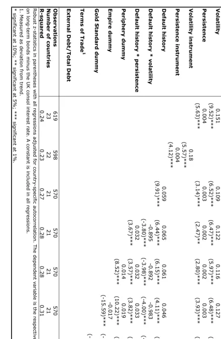
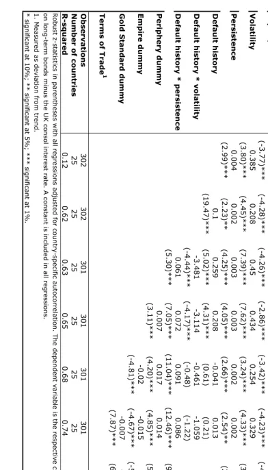
Starting with the HP-filter measure of cyclical persistence, Table 3 spans the pre-WWI era reporting the pooled OLS regressions of the country spread as the left-hand side variable. The country spread is defined as the (average) interest rate on the respective sovereign bonds relative to the benchmark foreign interest rate of similar maturity (the UK consol for the pre-WII period and the US long bond rate later – see Appendix 2). The reported z-statistics are corrected for heterocedasticity (using the standard White estimator) and for country-specific first-order auto-correlation. Debt to GDP, exports to GDP, volatility, and persistence enter the regression with a one-year lag so as to mitigate endogeneity biases.18 As in Obstfeld and Taylor (2003), we
drop from all regressions observations corresponding to spreads above 1,000 basis points so as to eliminate non-traded bonds and bonds of countries in default.
[Table 3 about here]
Column (1) in Table 3 reports our baseline specification without a de-fault premium term. This specification could be interpreted as testing the
17As can be seen from the above equation, how much the shock is attributed to the
trend vs. to the transient component in the BN decomposition depends on the persis-tence parameter ρ. In terms of our model, this amounts to assuming that there is just one shock but investors make inferences about ρ. Working, as we did, with two shocks and a common knowledge assumption about ρ facilitates the theoretical exposition and comparative statics. These approach are equivalent empirical strategies based on the BN decomposition.
18The external interest rate could be thought of as exogenous for all but two countries
in our sample – the US and the UK. However a specifications with rf lagged one year
symmetric information benchmark version of our model (where the default premium is zero), as well as variants found in other studies discussed above. As typical in country spread regressions, the R-square is relatively low reflect-ing the fact that spreads are known to be sensitive to news and uncorrelated shocks. Yet, all the estimated coefficients yield signs that are consistent with those of the theoretical model and are statistically significant at 5 percent, including the debt-to-GDP variable which was not found to be significant by Obstfeld and Taylor (2003) in their pre-WWI regressions.19 The respective
point estimates show that a one percentage point increase in the conditional volatility implies a 15 basis point increase in sovereign spreads, while a 10 percentage point increase in persistence raises spreads by 4 basis points, all else constant. These effects may appear small by the standards of the 1980s or 1990s, but not so in the pre-WWI context when the average spread was about 200 basis points and the cross-country dispersion of spreads was much tighter.20
In light of the potential endogeneity problems, column (2) of Table 3 replaces the output gap-based indicators with an instrument. In order to ensure strict exogeneity, and thus stack the deck against the postulated hy-potheses, we do not follow the usual approach of including weakly exogenous variables in the regressions creating these instruments; instead, we construct the country-specific instrument for the output gap indicator by regressing the latter of the respective country’s terms of trade, the world interest rate, and an indicator of world output growth.21 To the extent that these three
variables are strictly exogenous to individual country spreads, any remain-ing endogeneity bias is eliminated. The results of this instrumental variable regression clearly indicate the previous results were robust: all coefficients
19The discrepancy may be due to a variety of reasons. Obstfeld and Taylor (2003) do
not control for the volatility and persistence effects considered here; our sample has wider country coverage and for four Latin American countries uses GDP indicators that are deemed to be more reliable than the Maddison data used in their study. See Appendix 2 for details.
20Furthermore, cross-country spread dispersion declined dramatically during the period
as capital markets became more internationally integrated. By the eve of WWI, the cross-country standard deviation of spreads was down to 91 basis points. See Flandreau and Zumer (2004), for a discussion of these trends.
21These estimate of world output growth was constructed as a weighted average of real
retain a very similar order of magnitude of the regressions in column and are statistically significant at 1%.
Column (3) of Table 3 introduces a default history variable. This country-specific credit history indicator gauges how much of the default premium percolates into the country spread. In other words, we now test the extent to which the borrower’s action (default vs. repay) helps explain the evolution of spreads over and above the information contained in other fundamentals. Our indicator of default history is defined as the number of years in default since the beginning of the sample, so as to captures this time-dependence. As such, this boost to the spread from the default premium decays over time with successive repayments and bounces back up every time a new default occurs, as entailed by the model.22 As per Hypothesis 1, we expect this variable to be positively correlated with current spreads and statistically significant. Table 3 shows that this is the case. Its point estimate indicates that a country with a default history at the sample mean (0.08) has its spread boosted by over 40 basis points relative to a country that has never defaulted. Once again, since spreads for the 1870-1913 period averaged some 200 basis points, the effect was substantial. In particular, for those countries in the sample which spent up 30 percent of the time incurring arrears on foreign debt, the default premium could exceed 150 basis points.
Results reported in column (4) of Table 3 gauge the direction and extent to which the persistence and volatility of output interact with the default premium. Consistent with Hypothesis 2, conditional upon default, countries with higher persistence tend to have a higher default premium, boosting the respective country spread by another 25 basis points at mean (0.08*0.032) times the persistence parameter (0.5 on average). In contrast, the negative sign on the interactive volatility variable (default history*volatility) indicates that higher conditional output volatility tends to dampen the default pre-mium. This is consistent with the notion discussed in Section 2.5 that greater dispersion of output shocks tends to reduce the information content of de-fault/repayment actions and hence the default premium. It is also consistent with the idea that higher underlying output volatility makes default more excusable in the sense of Grossman and Van Huyck (1988); so spreads do not rise as much following a default announcement relative to baseline. In other words, even though the net effect of volatility on country spreads remain
itive,23 the asymmetric information mechanism working through the default
premium measure appears to be dampening this effect somewhat.
Columns (5) to (9) of Table 3 subject these findings to variety of con-trols. We start with fixed effects associated with differences between devel-oped countries and less develdevel-oped ones by introducing a “periphery” dummy, which takes a value one for countries in the periphery and zero otherwise (as in Obtsfeld and Taylor, 2003). The aim is to capture a host of structural characteristics not amenable to easy measurement, such as quality of insti-tutions and degrees of financial development. To the extent that quality of institutions and financial maturity are also proxies for the degree of informa-tion asymmetries, we should expect this catch-all variable to be significantly related to spreads and possibly weaken somewhat the coefficient on the de-fault history indicator. Our empirical results conforms with the theoretical priors.
We also introduce, as Obstfeld and Taylor (2003) did, an “empire” dummy that indicates if a country was part of the British empire – a catch-all proxy for assurances of greater investors’ legal protection and arguably better ac-cess to relevant country-specific information. In the context of our model, this dummy can be viewed as both capturing a a potential increase in the recovery rate parameterc, which will tend to lower spreads, and also a proxy for lower information asymmetries. As expected, this dummy takes on the expected negative sign, is highly significant statistically, and its inclusion in the regression lowers somewhat the coefficient on the default history variable. Exchange rate regimes are often perceived to be related to country risk, so it seems important to examine whether our hypotheses stand up to such a control variable. In the pre-WWII era, the main dichotomy is that be-tween countries that were on the gold standard and those that were not, so “Gold” dummy (taking on the unit value for those on the gold standard) was introduced. The results reported in column (5) are consistent with the findings of Bordo and Rockoff (1996) as well as Obstfeld and Taylor (2003): membership of the gold standard shaved off some 70 basis points in country spreads, consistent with the view of gold standard membership as a ‘good housekeeping seal of approval’. Its main effect in the regression is to lower
23This can be seen by multiplying the point estimate of 0.895 by the mean of the
the significance of the openness variable, without substantially affecting the size and statistical significance of the model’s variables of interest.
The remaining controls in the regressions are the ratio of foreign currency-denominated external debt to total debt (a proxy for ’original sin’, as in IADB, 2006), and terms of trade shock: if large enough, the latter may prompt a country into default along the lines of capacity to pay arguments. Neither of these variables are statistically significant. Nor do their inclusion impact on the proximate magnitude and statistical significance of volatility, persistence, and default premium terms. Overall, the results for the pre-WWI period are very consistent with the model’s theoretical priors and provide significant support for the hypotheses laid out above.
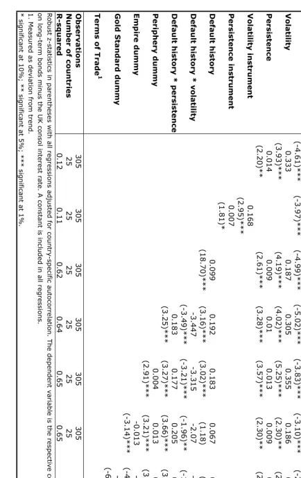
Table 4 turns to the interwar period. We follow Obstfeld and Taylor (2003) in focusing on the post-1924 years, thereby dropping from the sam-ple the early post-WWI spell – when war dislocations, hyperinflations, and Britain’s delay in re-joining gold had far-reaching effects on international bond issuance. As a result while the country coverage rises to 25 due to greater availability of output data, the number of observations is nearly half of the pre-WWI sample in Table 3. We follow the same empirical strategy as in Table 3, starting with the symmetric information baseline model, before adding the other variables and controls.
Column (1) in Table 4 indicates that the fit of the baseline model is much poorer than its pre-WWI counterpart. Neither the international risk free rate nor the debt to GDP ratio are statistically significant any longer at conventional levels though both retain their expected theoretical signs. As will be seen below, both features of this baseline regression will change drastically as we bring this stripped-down specification closer to our model. Even without doing so, the volatility and persistence indicators remain both significant at 5% and effect of persistence on spreads is now much larger: a 10 percentage point increase in persistence leads to 14 basis point increase in spreads (as opposed to 4 bps in the pre-WWI sample). Instrumenting both variables out as in column (2) halves the respective coefficients, but both variables remain significant at close to 5%.24
24This is partly related to the fact that, as most economies in our sample became closer
[Table 4 about here]
Column (3) in Table 4 shows that introducing default history has a major impact on the regression fit and also on the statistical significance of the debt to GDP ratio. This may not appear surprising since there were many defaults during this short period. However, the results signals the presence of a positive and large default premium; the existence of which has previously been disputed in the literature on the inter-War period (Eichengreen and Portes, 1989; Jorgensen and Sachs, 1989). Introducing the interactive term between the default history and persistence also brings out results that clearly support Hypotheses 1 and 3, and consistent with those of the pre-WWI sample.
These results remain basically the same after the introduction of a periph-ery dummy in column (5). However, once the empire dummy is introduced (column 6), its main effect is to bring down the significance of the default history variable. For the reasons discussed in connection with the pre-WWI regressions, this loss in the significance is not surprising: the empire dummy is also proxying for the existence of asymmetric information between borrowers and lenders and, if anything, differences in credit information and enforce-ment between empire and non-empire countries appear to have become par-ticularly stark in the inter-war era (Eichengreen and Portes, 1989). Further, this tighter multicollinearity effect between the empire dummy and default history should be expected once we take into account the short time span of the inter-war period. The fact that the overall fit of the regression does not change much after the introduction of the empire dummy corroborates this point. No less importantly, however, the coefficient on the stand-alone default history variable still retains the expected positive sign: its size and effect become stronger when interacted with the persistence indicator (the respective coefficient rising from 0.18 to 0.21). In short, once other controls related to the role of asymmetry of information are introduced in the regres-sion model, the main significant effect of default history on country spreads takes place via its interaction with the persistence parameter. Columns (7) and (8) corroborates these results, showing that they are robust to the in-clusion of a gold standard dummy and terms of trade shocks. Column (9)
drops the empire dummy while leaving in other controls, thus driving home the point about the collinearity effects between the default history history and the empire dummy over the inter-war sample.
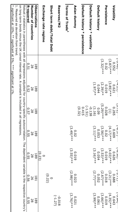
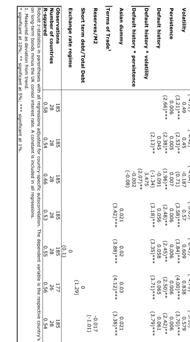
Table 5 reports the results for the 1994-2004 period. Despite the wider coverage in terms of number of countries, the number of observations in these regressions is considerably lower than the pre-WWII regressions due to the lack of bond spread data for many emerging markets before the late 1990s/early 2000s. The cross-sectional dimension of these regressions far dominates the time-series dimension. Partly reflecting this, the fit is much higher for the baseline regressions relative to the pre-War samples where the baseline model accounting for about half of variations in country spreads. Once again, the persistence and volatility variables are statistically signifi-cant as shown in column (1), so are the other two relevant model-dictated variables - the risk-free US interest rate and the debt-to-GDP ratio. Also consistent with our model, there is evidence of a positive and significant de-fault premium, as shown in column (3). This is so even though the 1994-2004 sample is severely biased toward countries that have defaulted serially in the past (mostly issuers of Brady bonds), excluding all advanced countries that were previously present in the two pre-WWII samples. Regression results reflect these two sample limitations – the very limited time-series dimen-sion and the bias towards countries that with higher output volatility and persistence that have default serially in the past. This can be seen from re-sults in column (4), which indicate substantial multicollinearity between the stand-alone default history variable and its interactive terms with conditional output volatility and persistence. Once the three variables are included in the regression, two of them are statistically insignificant and one of them (de-fault history*persistence) yields the opposite sign. Looking at the underlying raw data, the reason is clear: the correlation coefficients between default his-tory and the two interactive terms are 0.89 and 0.92 respectively. In other words, given the post-1993 sample limitations, not much new information can be drawn from such interactive terms once default history, persistence and volatility are already present in the regression. On this basis, we proceed by keeping the default history variable in the regression alone and gradually introduce new controls.
The first control pertains to the inclusion of regional dummies rather than a periphery dummy (given that these regressions encompass a more homogenous group of emerging markets), of which only the dummy for Asia is significant (column 4 of Table 5).25 In contrast with the pWWII
re-gressions, column 5 shows that the exchange rate regime does not matter for emerging market countries. Greater data availability for the post-1993 sample now allows us also to test the effects of debt maturity, terms of trade shocks, and international reserve coverage (as a share of broad money, M2), variables often deemed to be important in explaining financial and currency crises (Kaminsky and Reinhart, 1998). Results reported in columns (6) to (8) show that none of them adds to the model’s explanatory power on country risk. Finally, columns (9) and (10) drop the default history variable and enter only the respective interactive terms on volatility and persistence. In con-trast with pre-WWII results, the default history*volatility term now yields a positive sign. In contrast, persistence-default history interactive variable yields the model’s predicted sign and is statistically significant at 1%. Over-all, and taking into account the post-1993 sample limitations, we take the results as broadly consistent with the theoretical model and with Hypotheses 1 to 3.
We conclude this section by presenting a similar set of regressions using the Beveridge-Nelson (BN) measure of the “trend gap”. Since the ARIMA estimation is more data intensive and one needs longer data series to evalaute trend volatility and better distinguish between shocks to trend vs. shocks to cycle, we report such results only for the inter-war and the post-1993 samples.26 Starting with the interwar results in Table 6, two main differences
with the HP filter-measures of the output gap is that the coefficient on the stand-alone persistence is of an order of magnitude lower and that of volatility considerably higher. Since both sets of regressions span essentially the same observations, the difference seemingly lies on the BN filter’s attribution of
25This is likely because of Asian crisis governments in the late 1990s did not formally
go into default with the exception of Indonesia’s debt renegotiation but the havoc in these countries clearly weighed down on spreads.
26Results for the pre-WWI containing less than two-thirds of the observations featuring
output shocks to trend shocks, raising the persistence measure and hence lowering its estimated coefficient, all else constant. This result carries over to the default history-persistence interactive variable. Aside from this main difference, the results are closely in line with those of Table 4 using the HP-gap. This includes some of the dilution of the stand-alone default history variable when the empire dummy is introduced in the regressions, and the strong significance of default history when interacted with the persistence parameter. As in the HP-filter regressions of Table 4, the model’s other main predictions are robust to a variety of controls. Likewise, post-1993 results, presented in Table 7 are very similar with their HP-gap counterparts in Table 5.
[Table 6 and 7 about here]
Overall, we conclude from this section that the default trap pricing mech-anism postulated in our model is broadly consistent with long-run data on sovereign bond pricing and macroeconomic determinants. In particular, the roles of credit history and output persistence are generally highly significant and robust to a host of controls, including break-downs by period. Last but not least, our main empirical results are likewise robust to two classic de-trending methods, and not an artifact of HP-filter detrending.
4
Conclusion
History tells us that sovereign creditworthiness displays persistence: coun-tries that default once are more likely to do so again, and face higher spreads as a result. This paper has sought to rationalize this stylized fact through the idea of a default premium. A sovereign’s decision to default signals that it was likely hit by a large negative output shock which may persist, thus raising future debt-to-output ratios above the expected baseline. As compet-itive lenders seek to break even and the sovereign continues to tap the market given its financing needs, this gives rise to a positive default premium. By increasing country spreads, and hence the borrower’s debt burden relative to output, this mechanism makes future default more likely, thus creating default traps.
nature of output shocks – without it, the default premium is zero and spreads do not react to repayment decisions beyond publicly known information about fundamentals. Second, shocks to the gap between actual and ex-pected output (the “output gap”) must be reasonably persistent – without persistence default decisions have no informational content on the evolution of debt burden relative to output. Third, output must be sufficiently volatile, so that countries may face output realizations that are low enough to make default optimal.
While previous studies have examined the impact of output volatility and persistence on country spreads and default risk, none of them has, to the best of our knowledge, linked these ingredients together. As a result, while previ-ous theoretical models show that high conditional volatility and persistence of output shocks alone can explain serial default, they cannot account for why two countries with the same fundamentals (including underlying volatil-ity and persistence of output shocks) may face distinct spreads. In this paper, we show that this may happen if they suffer different output realizations at a given point in time that lead one – struck by an adverse shock – to default and the other to repay. Under asymmetric information, the defaulting coun-try will face higher spreads and hence a heavier debt burden in the future, so it is more likely to default again all else constant. As such, our model delivers path dependence in credit history in a way not discussed in previous work. Further, since default in our model reveals new forward-looking in-formation about debt burdens that supplements publicly-known inin-formation about fundamentals, our theoretical mechanism also explains the well-known fact that spreads shoot up following default announcements.
The other main contribution of this paper is empirical. Empirical testing of previous theoretical models of default risk has employed more limited data sets than ours. To test the postulated theoretical mechanism, this paper de-velops a comprehensive cross-country dataset spanning over a century. This is important because default history and the causal mechanisms postulated in our model display significant cross-country differences (due to institutions, commodity specialization, etc.) which are typically structural and hence slowly-evolving; so it is key that a thorough test of the theory be based on a broad cross-country sample with a reasonably long time series dimension.
volatil-ity and persistence of output gaps. Second, countries face a substantially positive and statistically significant default premium. Third, such a default premium is rising in the underlying persistence of output shocks. These re-sults are robust to a host of controls featuring in previous studies. They are also very robust to measures of output volatility and persistence based on distinct detrending methods. We interpret this empirical findings as strong evidence that the default trap mechanism postulated in our model is consis-tent with long-run data on sovereign bond pricing and the macroeconomic determinants. As such, our model provides an additional and complementary mechanism to those postulated in earlier work on the pervasiveness of serial default and “debt intolerance” (Reinhart et al., 2003). On the empirical side, our historical evidence also highlights the important role of historical output volatility and persistence indicators in country spread regressions, particu-larly for pre-WWII period where the inclusion of these variables has been regrettably absent in previous work.
References
1. Acemoglu D., S. Johnson and J. Robinson, 2005, “Institutions as the Fundamental Cause of Long-Run Growth,” in P. Aghion and S. Durlauf (eds.), Handbook of Economic Growth, North Holland: Amsterdam.
2. Aguiar, M. and G. Gopinath, 2006,“Defaultable Debt, Interest Rates and the Current Account,” Journal of International Economics, 69(1), 61-89.
3. Aguiar, M. and G. Gopinath, 2007, “Emerging Market Business Cycles: The Cycle is the Trend,” Journal of Political Economy, 115(1), 69-102
4. Aiolfi, M., L. Cat˜ao, and A. Timmermann, 2006, “Common Factors in Latin America’s Business Cycles,” IMF working paper 6/49.
5. Alfaro, L., and F. Kanczuk, 2005, “Sovereign Debt as a Contingent Claim: A Quantitative Approach,” Journal of International Economics, 65, 297-314.
6. Arellano, C., 2006, “Default Risk and Income Fluctuations in Emerging Economies,” mimeo, University of Minnesota.
7. Beveridge, S. and C. Nelson, 1981, “A New Approach to Decomposition of Economic Time Series into Permanent and Transitory Components,” Journal of Monetary Economics, 7, 151-74.
8. Blattman, C., J. Hwang, and J. Williamson, 2007, “Winners and Losers in the Commodity Lottery: The Impact of Trade Growth and Volatility in the Periphery 1870-1939,” 82(1), 156-179.
9. Bordo, M. and H. Rockoff, 1996,“The Gold Standard as a ‘Good House-keeping Seal of Approval’,” Journal of Economic History, 56, 389-428. 10. Bulow, J. and K. Rogoff, 1989, “A Constant Recontracting Model of
Sovereign Debt,” Journal of Political Economy, 97, 155-78.
12. Calvo, G., and C. Vegh, 1999, “Inflation Stabilization and BOP Crises in Developing Countries,” in John Taylor and Michael Woodford (eds.), Handbook of Macroeconomics, Volume C, North Holland, Amsterdam. 13. Calvo, G., and E. Mendoza, 2000, “Capital Markets Crises and Eco-nomic Collapse in Emerging Markets: An Informational Frictions Ap-proach,” American Economic Review, Papers and Proceedings, March. 14. Cashin, P., Liang, H. and McDermott, C. John, 2000, “How Persistent are Shocks to World Commodity Prices?,” IMF Staff Papers, 47, 177-217.
15. Cat˜ao, L., 2007, “Sudden Stops and Currency Drops: A Historical Look” in S. Edwards (ed.), The Decline of Latin American Economies: Growth, Institutions and Crises, University of Chicago Press.
16. Cat˜ao, L. and S. Kapur, 2006, “Volatility and the Debt Intolerance Paradox,” IMF Staff Papers, 56, 195-218.
17. Cohen, D., 1992, “Debt Crisis: A Post-Mortem,” NBER Macroeco-nomics Annual, National Bureau of Economic Research, Cambridge: Mass.
18. D’Erasmo, P., 2007, “Government Reputation and Debt Repayment in Emerging Economies,” mimeo, University of Texas at Austin.
19. Eaton, J., 1996, “Sovereign Debt, Reputation, and Credit Terms,” In-ternational Journal of Finance and Economics, 1, 25-36.
20. Eaton, J., and M. Gersovitz, 1981, “Debt with Potential Repudiation: Theoretical and Empirical Analysis,” Review of Economics and Statis-tics, 48, 284-309.
21. Eaton, J., and M. Gersovitz, 1995, “Some Curious Properties of a Fa-miliar Model of Debt and Default,” Economic Letters, 63, 367-371. 22. Eichengreen, B., and R. Portes, 1986, “Debt and Default in the 1930s:
Causes and Consequences,” European Economic Review, 30, 599-640. 23. Eichengreen, B., R. Hausmann, and U. Panizza, 2003, “Currency